Binary Packet Video Walkthrough

Here’s our 4th video walkthrough of some problems from last year’s Advent of Code. We had an in-depth code writeup back on Monday that you can check out. The video is here on YouTube, and you can also take a look at the code on GitHub!

If you’re enjoying this content, make sure to subscribe to our monthly newsletter! We’ll have some special offers coming out this month that you won’t want to miss!

Binary Packet Parsing

Today we're back with a new problem walkthrough, this time from Day 16 of last year's Advent of Code. In some sense, the parsing section for this problem is very easy - there's not much data to read from the file. In another sense, it's actually rather hard! This problem is about parsing a binary format, similar in some sense to how network packets work. It's a good exercise in handling a few different kinds of recursive cases.

As with the previous parts of this series, you can take a look at the code on GitHub here. This problem also has quite a few utilities, so you can observe those as well. This article is a deep-dive code walkthrough, so having the code handy to look at might be a good idea!

Problem Description

For this problem, we're decoding a binary packet. The packet is initially given as a hexadecimal string.

A0016C880162017C3686B18A3D4780

But we'll turn it into binary and start working strictly with ones and zeros. However, the decoding process gets complicated because the packet is structured in a recursive way. But let's go over some of the rules.

Packet Header

Every packet has a six-bit header. The first three bits give a "version number" for the packet. The next three bits give a "type ID". That part's easy.

Then there are a series of rules about the rest of the information in the packet.

Literals

If the type ID is 4, the packet is a "literal". We then parse the remainder of the packet in 5-bit chunks. The first bit tells us if it is the last chunk of the packet (0 means yes, 1 means there are more chunks). The four other bits in the chunk are used to construct the binary number that forms the "value" of the literal. The more chunks, the higher the number can be.

Operator Sizes

Packets that aren't literals are operators. This means they contain a variable number of subpackets.

Operators have one bit (after the 6-bit header) giving a "length" type. A length type of "1" tells us that the following 11 bits give the number of subpackets. If the length bit is "0", then the next 15 bits give the length of all the subpackets in bits.

The Packet Structure

We'll see how these work out as we parse them. But with this structure in mind, one thing we can immediately do is come up with a recursive data type for a packet. I ended up calling this PacketNode since I thought of each as a node in a tree. It's pretty easy to see how to do this. We start with a base constructor for a Literal packet that only stores the version and the packet value. Then we just add an Operator constructor that will have a list of subpackets as well as a field for the operator type.

data PacketNode =
  Literal Word8 Word64 |
  Operator Word8 Word8 [PacketNode]
  deriving (Show)

Once we've parsed the packet, the "questions to answer" are, for the easy part, to take the sum of all the packet versions in our packet, and then to actually calculate the packet value recursively for the hard part. When we get to that part, we'll see how we use the operators to determine the value.

Solution Approach

The initial "parsing" part of this problem is actually quite easy. But we can observe that even after we have our binary values, it's still a parsing problem! We'll have an easy enough time answering the question once we've parsed our input into a PacketNode. So the core of the problem is parsing the ones and zeros into our PacketNode.

Since this is a parsing problem, we can actually use Megaparsec for the second part, instead of only for getting the input out of the file. Here's a possible signature for our core function:

-- More on this type later
data Bit = One | Zero

parsePacketNode :: (MonadLogger m) => ParsecT Void [Bit] m PacketNode

Whereas we normally use Text as the second type parameter to ParsecT, we can also use any list type, and the library will know what to do! With this function, we'll eventually be able to break our solution into its different parts. But first, we should start with some useful helpers for all our binary parsing.

Binary Utilities

Binary logic comes up fairly often in Advent of Code, and there are quite a few different utilities we would want to use with these ones and zeros. We start with a data type to represent a single bit. For maximum efficiency, we'd want to use a BitVector, but we aren't too worried about that. So we'll make a simple type with two constructors.

data Bit = Zero | One
  deriving (Eq, Ord)

instance Show Bit where
  show Zero = "0"
  show One = "1"

Our first order of business is turning a hexadecimal character into a list of bits. Hexadecimal numbers encapsulate 4 bits. So, for example, 0 should be [Zero, Zero, Zero, Zero], 1 should be [Zero, Zero, Zero, One], and F should be [One, One, One, One]. This is a simple pattern match, but we'll also have a failure case.

parseHexChar :: (MonadLogger m) => Char -> MaybeT m [Bit]
parseHexChar '0' = return [Zero, Zero, Zero, Zero]
parseHexChar '1' = return [Zero, Zero, Zero, One]
parseHexChar '2' = return [Zero, Zero, One, Zero]
parseHexChar '3' = return [Zero, Zero, One, One]
parseHexChar '4' = return [Zero, One, Zero, Zero]
parseHexChar '5' = return [Zero, One, Zero, One]
parseHexChar '6' = return [Zero, One, One, Zero]
parseHexChar '7' = return [Zero, One, One, One]
parseHexChar '8' = return [One, Zero, Zero, Zero]
parseHexChar '9' = return [One, Zero, Zero, One]
parseHexChar 'A' = return [One, Zero, One, Zero]
parseHexChar 'B' = return [One, Zero, One, One]
parseHexChar 'C' = return [One, One, Zero, Zero]
parseHexChar 'D' = return [One, One, Zero, One]
parseHexChar 'E' = return [One, One, One, Zero]
parseHexChar 'F' = return [One, One, One, One]
parseHexChar c = logErrorN ("Invalid Hex Char: " <> pack [c]) >> mzero

If we wanted, we could also include lowercase, but this problem doesn't require it.

We also want to be able to turn a list of bits into a decimal number. We'll do this for a couple different sizes of numbers. For smaller numbers (8 bits or below), we might want to return a Word8. For larger numbers we can do Word64. Calculating the decimal number is a tail recursive process, where we track the accumulated sum and the current power of 2.

bitsToDecimal8 :: [Bit] -> Word8
bitsToDecimal8 bits = if length bits > 8
  then error ("Too long! Use bitsToDecimal64! " ++ show bits)
  else btd8 0 1 (reverse bits)
    where
      btd8 :: Word8 -> Word8 -> [Bit] -> Word8
      btd8 accum _ [] = accum
      btd8 accum mult (b : rest) = case b of
        Zero -> btd8 accum (mult * 2) rest
        One -> btd8 (accum + mult) (mult * 2) rest

bitsToDecimal64 :: [Bit] -> Word64
bitsToDecimal64 bits = if length bits > 64
  then error ("Too long! Use bitsToDecimalInteger! " ++ (show $ bits))
  else btd64 0 1 (reverse bits)
    where
      btd64 :: Word64 -> Word64 -> [Bit] -> Word64
      btd64 accum _ [] = accum
      btd64 accum mult (b : rest) = case b of
        Zero -> btd64 accum (mult * 2) rest
        One -> btd64 (accum + mult) (mult * 2) rest

Last of all, we should write a parser for reading a hexadecimal string from our file. This is easy, because Megaparsec already has a parser for a single hexadecimal character.

parseHexadecimal :: (MonadLogger m) => ParsecT Void Text m String
parseHexadecimal = some hexDigitChar

Basic Bit Parsing

With all these utilities in place, we can get started with parsing our list of bits. As mentioned above, we want a function that generally looks like this:

parsePacketNode :: (MonadLogger m) => ParsecT Void [Bit] m PacketNode

However, we need one extra nuance. Because we have one layer that will parse several consecutive packets based on the number of bits parsed, we should also return this number as part of our function. In this way, we'll be able to determine if we're done with the subpackets of an operator packet.

parsePacketNode :: (MonadLogger m) => ParsecT Void [Bit] m (PacketNode, Word64)

We'll also want a wrapper around this function so we can call it from a normal context with the list of bits as the input. This looks a lot like the existing utilities (e.g. for parsing a whole file). We use runParserT from Megaparsec and do a case-branch on the result.

parseBits :: (MonadLogger m) => [Bit] -> MaybeT m PacketNode
parseBits bits = do
  result <- runParserT parsePacketNode "Utils.hs" bits
  case result of
    Left e -> logErrorN ("Failed to parse: " <> (pack . show $ e)) >> mzero
    Right (packet, _) -> return packet

We ignore the "size" of the parsed packet in the primary case, but we'll use its result in the recursive calls to parsePacketNode!

Having done this, we can now start writing basic parser functions. To parse a single bit, we'll just wrap the anySingle combinator from Megaparsec.

parseBit :: ParsecT Void [Bit] m Bit
parseBit = anySingle

If we want to parse a certain number of bits, we'll want to use the monadic count combinator. Let's write a function that parses three bits and turns it into a Word8, since we'll need this for the packet version and type ID.

parse3Bit :: ParsecT Void [Bit] m Word8
parse3Bit = bitsToDecimal8 <$> count 3 parseBit

We can then immediately use this to start filling in our parsing function!

parsePacketNode :: (MonadLogger m) => ParsecT Void [Bit] m (PacketNode, Word64)
parsePacketNode = do
  packetVersion <- parse3Bit
  packetTypeId <- parse3Bit
  ...

Then the rest of the function will depend upon the different cases we might parse.

Parsing a Literal

We can start with the "literal" case. This parses the "value" contained within the packet. We need to track the number of bits we parse so we can use this result in our parent function!

parseLiteral :: ParsecT Void [Bit] m (Word64, Word64)

As explained above, we examine chunks 5 bits at a time, and we end the packet once we have a chunk that starts with 0. This is a "while" loop pattern, which suggests tail recursion as our solution!

We'll have two accumulator arguments. First, the series of bits that contribute to our literal value. Second, the number of bits we've parsed so far (which must include the signal bit).

parseLiteral :: ParsecT Void [Bit] m (Word64, Word64)
parseLiteral = parseLiteralTail [] 0
  where
    parseLiteralTail :: [Bit] -> Word64 -> ParsecT Void [Bit] m (Word64, Word64)
    parseLiteralTail accumBits numBits = do
      ...

First, we'll parse the leading bit, followed by the four bits in the chunk value. We append these to our previously accumulated bits, and add 5 to the number of bits parsed:

parseLiteral :: ParsecT Void [Bit] m (Word64, Word64)
parseLiteral = parseLiteralTail [] 0
  where
    parseLiteralTail :: [Bit] -> Word64 -> ParsecT Void [Bit] m (Word64, Word64)
    parseLiteralTail accumBits numBits = do
      leadingBit <- parseBit
      nextBits <- count 4 parseBit
      let accum' = accumBits ++ nextBits
      let numBits' = numBits + 5
      ...

If the leading bit is 0, we're done! We can return our value by converting our accumulated bits to decimal. Otherwise, we recurse with our new values.

parseLiteral :: ParsecT Void [Bit] m (Word64, Word64)
parseLiteral = parseLiteralTail [] 0
  where
    parseLiteralTail :: [Bit] -> Word64 -> ParsecT Void [Bit] m (Word64, Word64)
    parseLiteralTail accumBits numBits = do
      leadingBit <- parseBit
      nextBits <- count 4 parseBit
      let accum' = accumBits ++ nextBits
      let numBits' = numBits + 5
      if leadingBit == Zero
        then return (bitsToDecimal64 accum', numBits')
        else parseLiteralTail accum' numBits'

Then it's very easy to incorporate this into our primary function. We check the type ID, and if it's "4" (for a literal), we call this function, and return with the Literal packet constructor.

parsePacketNode :: (MonadLogger m) => ParsecT Void [Bit] m (PacketNode, Word64)
parsePacketNode = do
  packetVersion <- parse3Bit
  packetTypeId <- parse3Bit
  if packetTypeId == 4
    then do
      (literalValue, literalBits) <- parseLiteral
      return (Literal packetVersion literalValue, literalBits + 6)
    else
      ...

Now we need to consider the "operator" cases and their subpackets.

Parsing from Number of Packets

We'll start with the simpler of these two cases, which is when we are parsing a specific number of subpackets. The first step, of course, is to parse the length type bit.

parsePacketNode :: (MonadLogger m) => ParsecT Void [Bit] m (PacketNode, Word64)
parsePacketNode = do
  packetVersion <- parse3Bit
  packetTypeId <- parse3Bit
  if packetTypeId == 4
    then do
      (literalValue, literalBits) <- parseLiteral
      return (Literal packetVersion literalValue, literalBits + 6)
    else do
      lengthTypeId <- parseBit
      if lengthTypeId == One
        then do
        ...

First, we have to count out 11 bits and use that to determine the number of subpackets. Once we have this number, we just have to recursively call the parsePacketNode function the given number of times.

parsePacketNode :: (MonadLogger m) => ParsecT Void [Bit] m (PacketNode, Word64)
parsePacketNode = do
 ...
  if packetTypeId == 4
    then ...
    else do
      lengthTypeId <- parseBit
      if lengthTypeId == One
        then do
          numberOfSubpackets <- bitsToDecimal64 <$> count 11 parseBit
          subPacketsWithLengths <- replicateM (fromIntegral numberOfSubpackets) parsePacketNode
         ...

We'll unzip these results to get our list of packets and the lengths. To get our final packet length, we take the sum of the sizes, but we can't forget to add the header bits and the length type bit (7 bits), and the bits from the number of subpackets (11).

parsePacketNode :: (MonadLogger m) => ParsecT Void [Bit] m (PacketNode, Word64)
parsePacketNode = do
 ...
  if packetTypeId == 4
    then ...
    else do
      lengthTypeId <- parseBit
      if lengthTypeId == One
        then do
          numberOfSubpackets <- bitsToDecimal64 <$> count 11 parseBit
          subPacketsWithLengths <- replicateM (fromIntegral numberOfSubpackets) parsePacketNode
         let (subPackets, lengths) = unzip subPacketsWithLengths
          return (Operator packetVersion packetTypeId subPackets, sum lengths + 7 + 11)
        else

Parsing from Number of Bits

Parsing based on the number of bits in all the subpackets is a little more complicated, because we have more state to track. As we loop through the different subpackets, we need to keep track of how many bits we still have to parse. So we'll make a separate helper function.

parseForPacketLength :: (MonadLogger m) => Int -> Word64 -> [PacketNode] -> ParsecT Void [Bit] m ([PacketNode], Word64)
parseForPacketLength remainingBits accumBits prevPackets = ...

The base case comes when we have 0 bits remaining. Ideally, this occurs with exactly 0 bits. If it's a negative number, this is a problem. But if it's successful, we'll reverse the accumulated packets and return the number of bits we've accumulated.

parseForPacketLength :: (MonadLogger m) => Int -> Word64 -> [PacketNode] -> ParsecT Void [Bit] m ([PacketNode], Word64)
parseForPacketLength remainingBits accumBits prevPackets = if remainingBits <= 0
  then do
    if remainingBits < 0
      then error "Failing"
      else return (reverse prevPackets, accumBits)
  else ...

In the recursive case, we make one new call to parsePacketNode (the original function, not this helper). This gives us a new packet, and some more bits that we've parsed (this is why we've been tracking that number the whole time). So we can subtract the size from the remaining bits, and add it to the accumulated bits. And then we'll make the actual recursive call to this helper function.

parseForPacketLength :: (MonadLogger m) => Int -> Word64 -> [PacketNode] -> ParsecT Void [Bit] m ([PacketNode], Word64)
parseForPacketLength remainingBits accumBits prevPackets = if remainingBits <= 0
  then do
    if remainingBits < 0
      then error "Failing"
      else return (reverse prevPackets, accumBits)
  else do
    (newPacket, size) <- parsePacketNode
    parseForPacketLength (remainingBits - fromIntegral size) (accumBits + fromIntegral size) (newPacket : prevPackets)

And that's all! All our different pieces fit together now and we're able to parse our packet!

Solving the Problems

Now that we've parsed the packet into our structure, the rest of the problem is actually quite easy and fun! We've created a straightforward recursive structure, and so we can loop through it in a straightforward recursive way. We'll just always use the Literal as the base case, and then loop through the list of packets for the base case.

Let's start with summing the packet versions. This will return a Word64 since we could be adding a lot of package versions. With a Literal package, we just immediately return the version.

sumPacketVersions :: PacketNode -> Word64
sumPacketVersions (Literal v _) = fromIntegral v
...

Then with operator packets, we just map over the sub-packets, take the sum of their versions, and then add the original packet's version.

sumPacketVersions :: PacketNode -> Word64
sumPacketVersions (Literal v _) = fromIntegral v
sumPacketVersions (Operator v _ packets) = fromIntegral v +
  sum (map sumPacketVersions packets)

Now, for calculating the final packet value, we again start with the Literal case, since we'll just return its value. Note that we'll do this monadically, since we'll have some failure conditions in the later parts.

calculatePacketValue :: MonadLogger m => PacketNode -> MaybeT m Word64
calculatePacketValue (Literal _ x) = return x

Now, for the first time in the problem, we actually have to care what the operators mean! Here's a summary of the first few operators:

0 = Sum of all subpackets
1 = Product of all subpackets
2 = Minimum of all subpackets
3 = Maximum of all subpackets

There are three other operators following the same basic pattern. They expect exactly two subpackets and perform a binary, boolean operator. If it is true, the value is 1. If the operation is false, the packet value is 0.

5 = Greater than operator (<)
6 = Less than operator (>)
7 = Equals operator (==)

For the first set of operations, we can recursively calculate the value of the sub-packets, and take the appropriate aggregate function over the list.

calculatePacketValue :: MonadLogger m => PacketNode -> MaybeT m Word64
calculatePacketValue (Literal _ x) = return x
calculatePacketValue (Operator _ 0 packets) = sum <$> mapM calculatePacketValue packets
calculatePacketValue (Operator _ 1 packets) = product <$> mapM calculatePacketValue packets
calculatePacketValue (Operator _ 2 packets) = minimum <$> mapM calculatePacketValue packets
calculatePacketValue (Operator _ 3 packets) = maximum <$> mapM calculatePacketValue packets
...

For the binary operations, we first have to verify that there are only two packets.

calculatePacketValue :: MonadLogger m => PacketNode -> MaybeT m Word64
...
calculatePacketValue (Operator _ 5 packets) = do
  if length packets /= 2
    then logErrorN "> operator '5' must have two packets!" >> mzero
    else ...

Then we just de-structure the packets, calculate each value, compare them, and then return the appropriate value.

calculatePacketValue :: MonadLogger m => PacketNode -> MaybeT m Word64
...
calculatePacketValue (Operator _ 5 packets) = do
  if length packets /= 2
    then logErrorN "> operator '5' must have two packets!" >> mzero
    else do
      let [p1, p2] = packets
      v1 <- calculatePacketValue p1
      v2 <- calculatePacketValue p2
      return (if v1 > v2 then 1 else 0)
calculatePacketValue (Operator _ 6 packets) = do
  if length packets /= 2
    then logErrorN "< operator '6' must have two packets!" >> mzero
    else do
      let [p1, p2] = packets
      v1 <- calculatePacketValue p1
      v2 <- calculatePacketValue p2
      return (if v1 < v2 then 1 else 0)
calculatePacketValue (Operator _ 7 packets) = do
  if length packets /= 2
    then logErrorN "== operator '7' must have two packets!" >> mzero
    else do
      let [p1, p2] = packets
      v1 <- calculatePacketValue p1
      v2 <- calculatePacketValue p2
      return (if v1 == v2 then 1 else 0)
calculatePacketValue p = do
  logErrorN ("Invalid packet! " <> (pack . show $ p))
  mzero

Concluding Code

To tie everything together, we just follow the steps.

1. Parse the hexadecimal from the file
2. Transform the hexadecimal string into a list of bits
3. Parse the packet
4. Answer the question

For the first part, we use sumPacketVersions on the resulting packet.

solveDay16Easy :: String -> IO (Maybe Int)
solveDay16Easy fp = runStdoutLoggingT $ do
  hexLine <- parseFile parseHexadecimal fp
  result <- runMaybeT $ do
    bitLine <- concatMapM parseHexChar hexLine
    packet <- parseBits bitLine
    return $ sumPacketVersions packet
  return (fromIntegral <$> result)

And the "hard" solution is the same, except we use calculatePacketValue instead.

solveDay16Hard :: String -> IO (Maybe Int)
solveDay16Hard fp = runStdoutLoggingT $ do
  hexLine <- parseFile parseHexadecimal fp
  result <- runMaybeT $ do
    bitLine <- concatMapM parseHexChar hexLine
    packet <- parseBits bitLine
    calculatePacketValue packet
  return (fromIntegral <$> result)

And we're done!

Conclusion

That's all for this solution! As always, you can take a look at the code on GitHub. Later this week I'll have the video walkthrough as well. To keep up with all the latest news, make sure to subscribe to our monthly newsletter! Subscribing will give you access to our subscriber resources, like our Beginners Checklist and our Production Checklist.

Polymer Expansion Video Walkthrough

Earlier this week I did a write-up of the Day 14 Problem from Advent of Code 2021. Today, I’m releasing a video walkthrough that you can watch here on YouTube!

If you’re enjoying this content, make sure to subscribe to our monthly newsletter! This will give you access to our subscriber resources!

Polymer Expansion

Today we're back with another Advent of Code walkthrough. We're doing the problem from Day 14 of last year. Here are a couple previous walkthroughs:

1. Day 8 (Seven Segment Display)
2. Day 11 (Octopus Energy Levels)

If you want to see the code for today, you can find it here on GitHub!

If you're enjoying these problem overviews, make sure to subscribe to our monthly newsletter!

Problem Statement

The subject of today's problem is "polymer expansion". What this means in programming terms is that we'll be taking a string and inserting new characters into it based on side-by-side pairs.

The puzzle input looks like this:

NNCB

NN -> C
NC -> B
CB -> H
...

The top line of the input is our "starter string". It's our base for expansion. The lines that follow are codes that explain how to expand each pair of characters.

So in our original string of four characters (NNCB), there are three pairs: NN, NC, and CB. With the exception of the start and end characters, each character appears in two different pairs. So for each pair, we find the corresponding "insertion character" and construct a new string where all the insertion characters come between their parent pairs. The first pair gives us a C, the second pair gives us a new B, and the third pair gets us a new H.

So our string for the second step becomes: NCNBCHB. We'll then repeat the expansion a certain number of times.

For the first part, we'll run 10 steps of the expansion algorithm. For the second part, we'll do 40 steps. Each time, our final answer comes from taking the number of occurrences of the most common letter in the final string, and subtracting the occurrences of the least common letter.

Utilities

The main utility we'll end up using for this problem is an occurrence map. I decided to make this general idea for counting the number of occurrences of some item, since it's such a common pattern in these puzzles. The most generic alias we could have is a map where the key and value are parameterized, though the expectation is that i is an Integral type:

type OccMapI a i = Map a i

The most common usage is counting items up from 0. Since this is an unsigned, non-negative number, we would use Word.

type OccMap a = Map a Word

However, for today's problem, we're gonna be dealing with big numbers! So just to be safe, we'll use the unbounded Integer type, and make a separate type definition for that.

type OccMapBig a = Map a Integer

We can make a couple useful helper functions for this occurrence map. First, we can add a certain number value to a key.

addKey :: (Ord a, Integral i) => OccMapI a i -> a -> i -> OccMapI a i
addKey prevMap key count = case M.lookup key prevMap of
    Nothing -> M.insert key count prevMap
    Just x -> M.insert key (x + count) prevMap

We can add a specialization of this for "incrementing" a key, adding 1 to its value. We won't use this for today's solution, but it helps in a lot of cases.

incKey :: (Ord a, Integral i) => OccMapI a i -> a -> OccMapI a i
incKey prevMap key = addKey prevMap key 1

Now with our utilities out of the way, let's start parsing our input!

Parsing the Input

First off, let's define the result types of our parsing process. The starter string comes on the first line, so that's a separate String. But then we need to create a mapping between character pairs and the resulting character. We'll eventually want these in a HashMap, so let's make a type alias for that.

type PairMap = HashMap (Char, Char) Char

Now for parsing, we need to parse the start string, an empty line, and then each line of the code mapping.

Since most of the input is in the code mapping lines, let's do that first. Each line consists of parsing three characters, just separated by the arrow. This is very straightforward with Megaparsec.

parsePairCode :: (MonadLogger m) => ParsecT Void Text m (Char, Char, Char)
parsePairCode = do
  input1 <- letterChar
  input2 <- letterChar
  string " -> "
  output <- letterChar
  return (input1, input2, output)

Now let's make a function to combine these character tuples into the map. This is a nice quick fold:

buildPairMap :: [(Char, Char, Char)] -> HashMap (Char, Char) Char
buildPairMap = foldl (\prevMap (c1, c2, c3) -> HM.insert (c1, c2) c3 prevMap) HM.empty

The rest of our parsing function then parses the starter string and a couple newline characters before we get our pair codes.

parseInput :: (MonadLogger m) => ParsecT Void Text m (String, PairMap)
parseInput = do
  starterCode <- some letterChar
  eol >> eol
  pairCodes <- sepEndBy1 parsePairCode eol
  return (starterCode, buildPairMap pairCodes)

Then it will be easy enough to use our parseFile function from previous days. Now let's figure out our solution approach.

A Naive Approach

Now at first, the polymer expansion seems like a fairly simple problem. The root of the issue is that we have to write a function to run one step of the expansion. In principle, this isn't a hard function. We loop through the original string, two letters at a time, and gradually construct the new string for the next step.

One way to handle this would be with a tail recursive helper function. We could accumulate the new string (in reverse) through an accumulator argument.

runExpand :: (MonadLogger m)
  => PairMap
  -> String -- Accumulator
  -> String -- Remaining String
  -> m String

The "base case" of this function is when we have only one character left. In this case, we append it to the accumulator and reverse it all.

runExpand :: (MonadLogger m) => PairMap -> String -> String -> m String
runExpand pairMap accum [lastChar] = return $ reverse (lastChar : accum)

For the recursive case, we imagine we have at least two characters remaining. We'll look these characters up in our map. Then we'll append the first character and the new character to our accumulator, and then recurse on the remainder (including the second character).

runExpand :: (MonadLogger m) => PairMap -> String -> String -> m String
runExpand _ accum [lastChar] = return $ reverse (lastChar : accum)
runExpand pairMap accum (firstChar: secondChar : rest) = do
  let insertChar = pairMap HM.! (nextChar, secondChar)
  runExpand pairMap (insertChar : firstChar : accum) (secondChar : rest)

There are some extra edge cases we could handle here, but this isn't going to be how we solve the problem. The approach works...in theory. In practice though, it only works for a small number of steps. Why? Well the problem description gives a hint: This polymer grows quickly. In fact, with each step, our string essentially doubles in size - exponential growth!

This sort of solution is good enough for the first part, running only 10 steps. However, as the string gets bigger and bigger, we'll run out of memory! So we need something more efficient.

A Better Approach

The key insight here is that we don't actually care about the order of the letters in the string at any given time. All we really need to think about is the number of each kind of pair that is present. How does this work?

Well recall some of our basic code pairs from the top:

NN -> C
NC -> B
CB -> H
BN -> B

With the starter string like NNCB, we have one NN pair, an NC pair, and CB pair. In the next step, the NN pair generates two new pairs. Because a C is inserted between the N, we lose the NN pair but gain a NC pair and a CN pair. So after expansion the number of resulting NC pairs is 1, and the number of CN pairs is 1.

However, this is true of every NN pair within our string! Suppose we instead start off this with:

NNCBNN

Now there are two NN pairs, meaning the resulting string will have two NC pairs and two CN pairs, as you can see by taking a closer look at the result: NCNBCHBBNCN.

So instead of keeping the complete string in memory, all we need to do is use the "occurrence map" utility to store the number of each pair for our current state. So we'll keep folding over an object of type OccMapBig (Char, Char).

The first step of our solution then is to construct our initial mapping from the starter code. We can do this by folding through the starter string in a similar way to the example code in the naive solution. We one or zero characters are left in our "remainder", that's a base case and we can return the map.

-- Same signature as naive approach
expandPolymerLong :: (MonadLogger m) => Int -> String -> PairMap -> m (Maybe Integer)
expandPolymerLong numSteps starterCode pairMap = do
  let starterMap = buildInitialMap M.empty starterCode
  ...
  where
    buildInitialMap :: OccMapBig (Char, Char) -> String -> OccMapBig (Char, Char)
    buildInitialMap prevMap "" = prevMap
    buildInitialMap prevMap [_] = prevMap
   ...

Now for the recursive case, we have at least two characters remaining, so we'll just increment the value for the key formed by these characters!

-- Same signature as naive approach
expandPolymerLong :: (MonadLogger m) => Int -> String -> PairMap -> m (Maybe Integer)
expandPolymerLong numSteps starterCode pairMap = do
  let starterMap = buildInitialMap M.empty starterCode
  ...
  where
    buildInitialMap :: OccMapBig (Char, Char) -> String -> OccMapBig (Char, Char)
    buildInitialMap prevMap "" = prevMap
    buildInitialMap prevMap [_] = prevMap
    buildInitialMap prevMap (firstChar : secondChar : rest) = buildInitialMap (incKey prevMap (firstChar, secondChar)) (secondChar : rest)

The key point, of course, is how to expand our map each step, so let's do this next!

A New Expansion

To run a single step in our naive solution, we could use a tail-recursive helper to gradually build up the new string (the "accumulator") from the old string (the "remainder" or "rest"). So our type signature looked like this:

runExpand :: (MonadLogger m)
  => PairMap
  -> String -- Accumulator
  -> String -- Remainder
  -> m String

For our new expansion step, we're instead taking one occurrence map and transforming it into a new occurrence map. For convenience, we'll include an integer argument keeping track of which step we're on, but we won't need to use it in the function. We'll do all this within expandPolymerLong so that we have access to the PairMap argument.

expandPolymerLong :: (MonadLogger m) => Int -> String -> PairMap -> m (Maybe Integer)
expandPolymerLong numSteps starterCode pairMap = do
  ...
  where
    runStep ::(MonadLogger m) => OccMapBig (Char, Char) -> Int -> m (OccMapBig (Char, Char))
    runStep = ...

The runStep function has a simple idea behind it though. We gradually reconstruct our occurrence map by folding through the pairs in the previous map. We'll make a new function runExpand to act as the folding function.

expandPolymerLong :: (MonadLogger m) => Int -> String -> PairMap -> m (Maybe Integer)
expandPolymerLong numSteps starterCode pairMap = do
  ...
  where
    runStep ::(MonadLogger m) => OccMapBig (Char, Char) -> Int -> m (OccMapBig (Char, Char))
    runStep prevMap _ = foldM runExpand M.empty (M.toList prevMap)

    runExpand :: (MonadLogger m) => OccMapBig (Char, Char) -> ((Char, Char), Integer) -> m (OccMapBig (Char, Char))
    runExpand = ...

For this function, we begin by looking up the two-character code in our map. If for whatever reason it doesn't exist, we'll move on, but it's worth logging an error message since this isn't supposed to happen.

runExpand :: (MonadLogger m) => OccMapBig (Char, Char) -> ((Char, Char), Integer) -> m (OccMapBig (Char, Char))
runExpand prevMap (code@(c1, c2), count) = case HM.lookup code pairMap of
  Nothing -> logErrorN ("Missing Code: " <> pack [c1, c2]) >> return prevMap
  Just newChar -> ...

Now once we've found the new character, we'll create our first new pair and our second new pair by inserting the new character with our previous characters.

runExpand :: (MonadLogger m) => OccMapBig (Char, Char) -> ((Char, Char), Integer) -> m (OccMapBig (Char, Char))
runExpand prevMap (code@(c1, c2), count) = case HM.lookup code pairMap of
  Nothing -> logErrorN ("Missing Code: " <> pack [c1, c2]) >> return prevMap
  Just newChar -> do
    let first = (c1, newChar)
        second = (newChar, c2)
  ...

And to wrap things up, we add the new count value for each of our new keys to the existing map! This is done with nested calls to addKey on our occurrence map.

runExpand :: (MonadLogger m) => OccMapBig (Char, Char) -> ((Char, Char), Integer) -> m (OccMapBig (Char, Char))
runExpand prevMap (code@(c1, c2), count) = case HM.lookup code pairMap of
  Nothing -> logErrorN ("Missing Code: " <> pack [c1, c2]) >> return prevMap
  Just newChar -> do
    let first = (c1, newChar)
        second = (newChar, c2)
  return $ addKey (addKey prevMap first count) second count

Rounding Up

Now we have our last task: finding the counts of the characters in the final string, and subtracting the minimum from the maximum. This requires us to first disassemble our mapping of pair counts into a mapping of individual character counts. This is another fold step. But just like before, we use nested calls to addKey on an occurrence map! See how countChars works below:

expandPolymerLong :: (MonadLogger m) => Int -> String -> PairMap -> m (Maybe Integer)
expandPolymerLong numSteps starterCode pairMap = do
  let starterMap = buildInitialMap M.empty starterCode
  finalOccMap <- foldM runStep starterMap [1..numSteps]
  let finalCharCountMap = foldl countChars M.empty (M.toList finalOccMap)
  ...
  where
    countChars :: OccMapBig Char -> ((Char, Char), Integer) -> OccMapBig Char
    countChars prevMap ((c1, c2), count) = addKey (addKey prevMap c1 count) c2 count

So we have a count of the characters in our final string...sort of. Recall that we added characters for each pair. Thus the number we're getting is basically doubled! So we want to divide each value by 2, with the exception of the first and last characters in the string. If these are the same, we have an edge case. We divide the number by 2 and then add an extra one. Otherwise, if a character has an odd value, it must be on the end, so we divide by two and round up. We sum up this logic with the quotRoundUp function, which we apply over our finalCharCountMap.

expandPolymerLong :: (MonadLogger m) => Int -> String -> PairMap -> m (Maybe Integer) expandPolymerLong numSteps starterCode pairMap = do let starterMap = buildInitialMap M.empty starterCode finalOccMap <- foldM runStep starterMap [1..numSteps] let finalCharCountMap = foldl countChars M.empty (M.toList finalOccMap) let finalCounts = map quotRoundUp (M.toList finalCharCountMap) ... where quotRoundUp :: (Char, Integer) -> Integer quotRoundUp (c, i) = if even i then quot i 2 + if head starterCode == c && last starterCode == c then 1 else 0 else quot i 2 + 1

And finally, we consider the list of outcomes and take the maximum minus the minimum!

```haskell
expandPolymerLong :: (MonadLogger m) => Int -> String -> PairMap -> m (Maybe Integer)
expandPolymerLong numSteps starterCode pairMap = do
  let starterMap = buildInitialMap M.empty starterCode
  finalOccMap <- foldM runStep starterMap [1..numSteps]
  let finalCharCountMap = foldl countChars M.empty (M.toList finalOccMap)
  let finalCounts = map quotRoundUp (M.toList finalCharCountMap)
  if null finalCounts
    then logErrorN "Final Occurrence Map is empty!" >> return Nothing
    else return $ Just $ fromIntegral (maximum finalCounts - minimum finalCounts)

  where
    buildInitialMap = ...
    runStep = ...
    runExpand = ...
    countChars = ...
    quotRoundUp = ...

Last of all, we combine input parsing with solving the problem. Our "easy" and "hard" solutions look the same, just with different numbers of steps.

solveDay14Easy :: String -> IO (Maybe Integer)
solveDay14Easy fp = runStdoutLoggingT $ do
  (starterCode, pairCodes) <- parseFile parseInput fp
  expandPolymerLong 10 starterCode pairCodes

solveDay14Hard :: String -> IO (Maybe Integer)
solveDay14Hard fp = runStdoutLoggingT $ do
  (starterCode, pairCodes) <- parseFile parseInput fp
  expandPolymerLong 40 starterCode pairCodes

Conclusion

Hopefully that solution makes sense to you! In case I left anything out of my solution, you can peruse the code on GitHub. Later this week, we'll have a video walkthrough of this solution!

If you're enjoying this content, make sure to subscribe to our monthly newsletter, which will also give you access to our Subscriber Resources!

Dijkstra Video Walkthrough

Today I’m taking a really quick break from Advent of Code videos to do a video walkthrough of Dijkstra’s algorithm! I did several written walkthroughs of this algorithm a couple months ago:

1. Basic Algorithm

2. Generalizing with a Typeclass

3. Generalizing with Type Families

4. Applying to a 2D Grid

5. Comparing to the Library Function

6. Using a Monad

However, I never did a video walkthrough on my YouTube channel, and a viewer specifically requested one, so here it is today!

If you enjoyed that video, make sure to subscribe to our monthly newsletter so you can stay up to date on our latest content! This will also give you access to our subscriber resources!

Octopus Energy - Video Walkthrough

Here’s another Video walkthrough, which you can find here on YouTube. This is for the Day 11 problem. You can find a detailed written walkthrough here. The code is also available on GitHub.

There will be one non-Advent-of-Code video later this week, and then next week we’ll be back with more problem solving walkthroughs!

Seven Segment Display - Video Walkthrough

As promised, today I’m back on YouTube, releasing a video walkthrough of my solution to the Seven Segment Display problem that we went over last week in this detailed blog post.

Next week I’ll be following up with another video walkthrough, this time for Day 11 that we covered earlier this week! Make sure to subscribe if you’re enjoying this content!

Flashing Octopuses and BFS

Today we continue our new series on Advent of Code solutions from 2021. Last time we solved the seven-segment logic puzzle. Today, we'll look at the Day 11 problem which focuses a bit more on traditional coding structures and algorithms.

This will be another in-depth coding write-up. For the next week or so after this I'll switch to doing video reviews so you can compare the styles. I haven't been too exhaustive with listing imports in these examples though, so if you're curious about those you can take a look at the full solution here on GitHub. So now, let's get started!

Problem Statement

For this problem, we're dealing with a set of Octopuses, (Advent of Code had an aquatic theme last year) and these octopuses apparently have an "energy level" and eventually "flash" when they reach their maximum energy level. They sit nicely in a 2D grid for us, and the puzzle input is just a grid of single-digit integers for their initial "energy level". Here's an example.

5483143223
2745854711
5264556173
6141336146
6357385478
4167524645
2176841721
6882881134
4846848554
5283751526

Now, as time goes by, their energy levels increase. With each step, all energy levels go up by one. So after a single step, the energy grid looks like this:

6594254334
3856965822
6375667284
7252447257
7468496589
5278635756
3287952832
7993992245
5957959665
6394862637

However, when an octopus reaches level 10, it flashes. This has two results for the next step. First, its own energy level always reverts to 0. Second, it increments the energy level of all neighbors as well. This, of course, can make things more complicated, because we can end up with a cascading series of flashes. Even an octopus that has a very low energy level at the start of a step can end up flashing. Here's an example.

Start:
11111
19891
18181
19891
11111

End:
34543
40004
50005
40004
34543

The 1 in the center still ends up flashing. It has four neighbors as 9 which all flash. The surrounding 8's then flash because each has two 9 neighbors. As a result, the 1 has 8 neighbors flashing. Combining with its own increment, it becomes as 10, so it also flashes.

The good news is that all flashing octopuses revert to 0. They don't start counting again from other adjacent flashes so we can't get an infinite loop of flashing and we don't have to worry about the "order" of flashing.

For the first part of the problem, we have to find the total number of flashes after a certain number of steps. For the second part, we have to find the first step when all of the octopuses flash.

Solution Approach

There's nothing too difficult about the solution approach here. Incrementing the grid and finding the initial flashes are easy problems. The only tricky part is cascading the flashes. For this, we need a Breadth-First-Search where each item in the queue is a flash to resolve. As long as we're careful in our accounting and in the update step, we should be able to answer the questions fairly easily.

Utilities

As with last time, we'll start the coding portion with a few utilities that will (hopefully) end up being useful for other problems. The first of these is a simple one. We'll use a type synonym Coord2 to represent a 2D integer coordinate.

type Coord2 = (Int, Int)

Next, we'll want another general parsing function. Last time, we covered parseLinesFromFile, which took a general parser and applied it to every line of an input file. But we also might want to incorporate the "line-by-line" behavior into our general parser, so we'll add a function to parse the whole file given a single ParsecT expression. The structure is much the same, it just does even less work than our prior example.

parseFile :: (MonadIO m) => ParsecT Void Text m a -> FilePath -> m a
parseFile parser filepath = do
  input <- pack <$> liftIO (readFile filepath)
  result <- runParserT parser "Utils.hs" input
  case result of
    Left e -> error $ "Failed to parse: " ++ show e
    Right x -> return x

Last of all, this problem deals with 2D grids and spreading out the "effect" of one square over all eight of its neighbors. So let's write a function to get all the adjacent coordinates of a tile. We'll call this neighbors8, and it will be very similar to a function getting neighbors in 4 directions that I used in this Dijkstra's algorithm implementation.

getNeighbors8 :: HashMap Coord2 a -> Coord2 -> [Coord2]
getNeighbors8 grid (row, col) = catMaybes
  [maybeUp, maybeUpRight, maybeRight, maybeDownRight, maybeDown, maybeDownLeft, maybeLeft, maybeUpLeft]
  where
    (maxRow, maxCol) = maximum $ HM.keys grid
    maybeUp = if row > 0 then Just (row - 1, col) else Nothing
    maybeUpRight = if row > 0 && col < maxCol then Just (row - 1, col + 1) else Nothing
    maybeRight = if col < maxCol then Just (row, col + 1) else Nothing
    maybeDownRight = if row < maxRow && col < maxCol then Just (row + 1, col + 1) else Nothing
    maybeDown = if row < maxRow then Just (row + 1, col) else Nothing
    maybeDownLeft = if row < maxRow && col > 0 then Just (row + 1, col - 1) else Nothing
    maybeLeft = if col > 0 then Just (row, col - 1) else Nothing
    maybeUpLeft = if row > 0 && col > 0 then Just (row - 1, col - 1) else Nothing

This function could also apply to an Array instead of a Hash Map. In fact, it might be even more appropriate there. But below we'll get into the reasons for using a Hash Map.

Parsing the Input

Now, let's get to the first step of the problem itself, which is to parse the input. In this case, the input is simply a 2D array of single-digit integers, so this is a fairly straightforward process. In fact, I figured this whole function could be re-used as well, so it could also be considered a utility.

The first step is to parse a line of integers. Since there are no spaces and no separators, this is very simple using some.

import Data.Char (digitToInt)
import Text.Megaparsec (some)

parseDigitLine :: ParsecT Void Text m [Int]
parseDigitLine = fmap digitToInt <$> some digitChar

Now getting a repeated set of these "integer lists" over a series of lines uses the same trick we saw last time. We use sepEndBy1 combined with the eol parser for end-of-line.

parse2DDigits :: (Monad m) => ParsecT Void Text m [[Int]]
parse2DDigits = sepEndBy1 parseDigitLine eol

However, we want to go one step further. A list-of-lists-of-ints is a cumbersome data structure. We can't really update it efficiently. Nor, in fact, can we even access 2D indices quickly. There are two good structures for us to use, depending on the problem. We can either use a 2D array, or a HashMap where the keys are 2D coordinates.

Because we'll be updating the structure itself, we want a Hash Map in this case. Haskell's Array structure has no good way to update its values without a full copy. If the structure were read only though, Array would be the better choice. For our current problem, the mutable array pattern would also be an option. But for now I'll keep things simpler.

So we need a function to convert nested integer lists into a Hash Map with coordinates. The first step in this process is to match each list of integers with a row number, and each integer within the list with its column number. Infinite lists, ranges and zip are excellent tools here!

hashMapFromNestedLists :: [[Int]] -> HashMap Coord2 Int
hashMapFromNestedLists inputs = ...
  where
    x = zip [0,1..] (map (zip [0,1..]) inputs)

Now in most languages, we would use a nested for-loop. The outer structure would cover the rows, the inner structure would cover the columns. In Haskell, we'll instead do a 2-level fold. The outer layer (the function f) will cover the rows. The inner layer (function g) will cover the columns. Each step updates the Hash Map appropriately.

hashMapFromNestedLists :: [[Int]] -> HashMap Coord2 Int
hashMapFromNestedLists inputs = foldl f HM.empty x
  where
    x = zip [0,1..] (map (zip [0,1..]) inputs)

    f :: HashMap Coord2 Int -> (Int, [(Int, Int)]) -> HashMap Coord2 Int
    f prevMap (row, pairs) = foldl (g row) prevMap pairs

    g :: Int -> HashMap Coord2 Int -> Coord2 -> HashMap Coord2 Int
    g row prevMap (col, val) = HM.insert (row, col) val prevMap

And now we can pull it all together and parse our input!

solveDay11Easy :: String -> IO (Maybe Int)
solveDay11Easy fp = do
  initialState <- parseFile parse2DDigitHashMap fp
  ...

solveDay11Hard :: String -> IO (Maybe Int)
solveDay11Hard fp = do
  initialState <- parseFile parse2DDigitHashMap fp
  ...

Basic Step Running

Now let's get to the core of the algorithm. The function we really need to get right here is a function to update a single step of the process. This will take our grid as an input and produce the new grid as an output, as well as some extra information. Let's start by making another type synonym for OGrid as the "Octopus grid".

type OGrid = HashMap Coord2 Int

Now a simple version of this function would have a type signature like this:

runStep :: (MonadLogger m) => OGrid -> m OGrid

(As mentioned last time, I'm defaulting to using MonadLogger for most implementation details).

However, we'll include two extra outputs for this function. First, we want an Int for the number of flashes that occurred on this step. This will help us with the first part of the problem, where we are summing the number of flashes given a certain number of steps.

Second, we want a Bool indicating that all of them have flashed. This is easy to derive from the number of flashes and will be our terminal condition flag for the second part of the problem.

runStep :: (MonadLogger m) => OGrid -> m (OGrid, Int, Bool)

Now the first thing we can do while stepping is to increment everything. Once we've done that, it is easy to pick out the coordinates that ought be our "initial flashes" - all the items where the value is at least 10.

runStep :: (MonadLogger m) => OGrid -> m (OGrid, Int, Bool)
runStep = ...
  where
  -- Start by incrementing everything
    incrementedGrid = (+1) <$> inputGrid
    initialFlashes = fst <$> filter (\(_, x) -> x >= 10) (HM.toList incrementedGrid)

Now what do we do with our initial flashes to propagate them? Let's defer this to a helper function, processFlashes. This will be where we perform the BFS step recursively. Using BFS requires a queue and a visited set, so we'll want these as arguments to our processing function. Its result will be the final grid, updated with all the incrementing done by the flashes, as well as the final set of all flashes, including the original ones.

processFlashes :: (MonadLogger m) =>
  HashSet Coord2 -> Seq Coord2 -> OGrid -> m (HashSet Coord2, OGrid)

In calling this from our runStep function, we'll prepopulate the visited set and the queue with the initial group of flashes, as well as passing the "incremented" grid.

runStep :: (MonadLogger m) => OGrid -> m (OGrid, Int, Bool)
runStep = do
  (allFlashes, newGrid) <- processFlashes (HS.fromList initialFlashes) (Seq.fromList initialFlashes) incrementedGrid
  ...
  where
  -- Start by incrementing everything
    incrementedGrid = (+1) <$> inputGrid
    initialFlashes = fst <$> filter (\(_, x) -> x >= 10) (HM.toList incrementedGrid)

Now the last thing we need to do is count the total number of flashes and reset all flashes coordinates to 0 before returning. We can also compare the number of flashes to the size of the hash map to see if they all flashed.

runStep :: (MonadLogger m) => OGrid -> m (OGrid, Int, Bool)
runStep inputGrid = do
  (allFlashes, newGrid) <- processFlashes (HS.fromList initialFlashes) (Seq.fromList initialFlashes) incrementedGrid
  let numFlashes = HS.size allFlashes
  let finalGrid = foldl (\g c -> HM.insert c 0 g) newGrid allFlashes
  return (finalGrid, numFlashes, numFlashes == HM.size inputGrid)
  where
  -- Start by incrementing everything
    incrementedGrid = (+1) <$> inputGrid
    initialFlashes = fst <$> filter (\(_, x) -> x >= 10) (HM.toList incrementedGrid)

Processing Flashes

So now we need to do this flash processing! To re-iterate, this is a BFS problem. We have a queue of coordinates that are flashing. In order to process a single flash, we increment its neighbors and, if incrementing puts its energy over 9, add it to the back of the queue to be processed.

So our inputs are the sequence of coordinates to flash, the current grid, and a set of coordinates we've already visited (since we want to avoid "re-flashing" anything).

processFlashes :: (MonadLogger m) =>
  HashSet Coord2 -> Seq Coord2 -> OGrid -> m (HashSet Coord2, OGrid)

We'll start with a base case. If the queue is empty, we'll return the input grid and the current visited set.

import qualified Data.Sequence as Seq
import qualified Data.HashSet as HS
import qualified Data.HashMap.Strict as HM

processFlashes :: (MonadLogger m) =>
  HashSet Coord2 -> Seq Coord2 -> OGrid -> m (HashSet Coord2, OGrid)
processFlashes visited queue grid = case Seq.viewl queue of
  Seq.EmptyL -> return (visited, grid)
  ...

Now suppose we have a non-empty queue and we can pull off the top element. We'll start by getting all 8 neighboring coordinates in the grid and incrementing their values. There's no harm in re-incrementing coordinates that have flashed already, because we'll just reset everything

processFlashes :: (MonadLogger m) =>
  HashSet Coord2 -> Seq Coord2 -> OGrid -> m (HashSet Coord2, OGrid)
processFlashes visited queue grid = case Seq.viewl queue of
  Seq.EmptyL -> return (visited, grid)
  top Seq.:< rest -> do
    -- Get the 8 adjacent coordinates in the 2D grid
    let allNeighbors = getNeighbors8 grid top
        -- Increment the value of all neighbors
        newGrid = foldl (\g c -> HM.insert c ((g HM.! c) + 1) g) grid allNeighbors
        ...

Then we want to filter this neighbors list down to the neighbors we'll add to the queue. So we'll make a predicate shouldAdd that tells us if a neighboring coordinate is a.) at least energy level 9 (so incrementing it causes a flash) and b.) that it is not yet visited. This lets us construct our new visited set and the final queue.

processFlashes :: (MonadLogger m) =>
  HashSet Coord2 -> Seq Coord2 -> OGrid -> m (HashSet Coord2, OGrid)
processFlashes visited queue grid = case Seq.viewl queue of
  Seq.EmptyL -> return (visited, grid)
  top Seq.:< rest -> do
    let allNeighbors = getNeighbors8 grid top
        newGrid = foldl (\g c -> HM.insert c ((g HM.! c) + 1) g) grid allNeighbors
        neighborsToAdd = filter shouldAdd allNeighbors
        newVisited = foldl (flip HS.insert) visited neighborsToAdd
        newQueue = foldl (Seq.|>) rest neighborsToAdd
    ...
  where
    shouldAdd :: Coord2 -> Bool
    shouldAdd coord = grid HM.! coord >= 9 && not (HS.member coord visited)

And, the cherry on top, we just have to make our recursive call with the new values.

processFlashes :: (MonadLogger m) =>
  HashSet Coord2 -> Seq Coord2 -> OGrid -> m (HashSet Coord2, OGrid)
processFlashes visited queue grid = case Seq.viewl queue of
  Seq.EmptyL -> return (visited, grid)
  top Seq.:< rest -> do
    let allNeighbors = getNeighbors8 grid top
        newGrid = foldl (\g c -> HM.insert c ((g HM.! c) + 1) g) grid allNeighbors
        neighborsToAdd = filter shouldAdd allNeighbors
        newVisited = foldl (flip HS.insert) visited neighborsToAdd
        newQueue = foldl (Seq.|>) rest neighborsToAdd
    processFlashes newVisited newQueue newGrid
  where
    shouldAdd :: Coord2 -> Bool
    shouldAdd coord = grid HM.! coord >= 9 && not (HS.member coord visited)

With processing done, we have completed our function for running a sinigle step.

Easy Solution

Now that we can run a single step, all that's left is to answer the questions! For the first (easy) part, we just want to count the number of flashes that occur over 100 steps. This will follow a basic recursion pattern, where one of the arguments tells us how many steps are left. The stateful values that we're recursing on are the grid itself, which updates each step, and the sum of the number of flashes.

runStepCount :: (MonadLogger m) => Int -> (OGrid, Int) -> (OGrid, Int)

Let's start with a base case. When we have 0 steps left, we return the inputs as the result.

runStepCount :: (MonadLogger m) => Int -> (OGrid, Int) -> m (OGrid, Int)
runStepCount 0 results = return results
...

The recursive case is also quite easy. We invoke runStep to get the updated grid and the number of flashses, and then recurse with a reduced step count, adding the new flashes to our previous sum.

runStepCount :: (MonadLogger m) => Int -> (OGrid, Int) -> m (OGrid, Int)
runStepCount 0 results = return results
runStepCount i (grid, prevFlashes) = do
  (newGrid, flashCount, _) <- runStep grid
  runStepCount (i - 1) (newGrid, flashCount + prevFlashes)

And then we can call this from our "easy" entrypoint:

solveDay11Easy :: String -> IO (Maybe Int)
solveDay11Easy fp = do
  initialState <- parseFile parse2DDigitHashMap fp
  (_, numFlashes) <- runStdoutLoggingT $ runStepCount 100 (initialState, 0)
  return $ Just numFlashes

Hard Solution

For the second part of the problem, we want to find the first step where *all octopuses flash**. Obviously once they synchronize the first time, they'll remain synchronized forever after that. So we'll write a slightly different recursive function, this time counting up instead of down.

runTillAllFlash :: (MonadLogger m) => OGrid -> Int -> m Int
runTillAllFlash inputGrid thisStep = ...

Each time we run this function, we'll call runStep. The terminal condition is when the Bool flag we get from runStep becomes true. In this case, we return the current step value.

runTillAllFlash :: (MonadLogger m) => OGrid -> Int -> m Int
runTillAllFlash inputGrid thisStep = do
  (newGrid, _, allFlashed) <- runStep inputGrid
  if allFlashed
    then return thisStep
    ...

Otherwise, we just going to recurse, except with an incremented step count.

runTillAllFlash :: (MonadLogger m) => OGrid -> Int -> m Int
runTillAllFlash inputGrid thisStep = do
  (newGrid, _, allFlashed) <- runStep inputGrid
  if allFlashed
    then return thisStep
    else runTillAllFlash newGrid (thisStep + 1)

And once again, we wrap up by calling this function from our "hard" entrypoint.

solveDay11Hard :: String -> IO (Maybe Int)
solveDay11Hard fp = do
  initialState <- parseFile parse2DDigitHashMap fp
  firstAllFlash <- runStdoutLoggingT $ runTillAllFlash initialState 1
  return $ Just firstAllFlash

And now we're done! Our program should be able to solve both parts of the problem!

Conclusion

For the next couple articles, I'll be walking through these same problems, except in video format! So stay tuned for that, and make sure you're subscribed to the YouTube channel so you get notifications about it!

And if you're interested in staying up to date with all the latest news on Monday Morning Haskell, make sure to subscribe to our mailing list. This will get you our monthly newsletter, access to our resources page, and you'll also get special offers on all of our video courses!

Advent of Code: Seven Segment Logic Puzzle

We're into the last quarter of the year, and this means Advent of Code is coming up again in a couple months! I'm hoping to do a lot of these problems in Haskell again and this time do up-to-date recaps. To prepare for this, I'm going back through my solutions from last year and trying to update them and come up with common helpers and patterns that will be useful this year.

You can follow me doing these implementation reviews on my stream, and you can take a look at my code on GitHub here!

Most of my blog posts for the next few weeks will recap some of these problems. I'll do written summaries of solutions as well as video summaries to see which are more clear. The written summaries will use the In-Depth Coding style, so get ready for a lot of code! As a final note, you'll notice my frequent use of MonadLogger, as I covered in this article. So let's get started!

Problem Statement

I'm going to start with Day 8 from last year, which I found to be an interesting problem because it was more of a logic puzzle than a traditional programming problem. The problem starts with the general concept of a seven segment display, a way of showing numbers on an electronic display (like scoreboards, for example).

We can label each of the seven segments like so, with letters "a" through "g":

Segments a-g:

     aaaa 
    b    c
    b    c
     dddd 
    e    f
    e    f
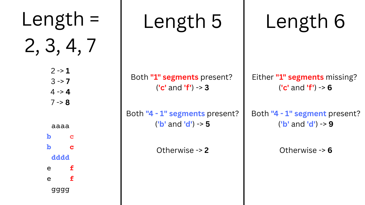
     gggg

If all seven segments are lit up, this indicates an 8. If only "c" and "f" are lit up, that's 1, and so on.

The puzzle input consists of lines with 10 "code" strings, and 4 "output" strings, separated by a pipe delimiter:

be cfbegad cbdgef fgaecd cgeb fdcge agebfd fecdb fabcd edb | fdgacbe cefdb cefbgd gcbe
edbfga begcd cbg gc gcadebf fbgde acbgfd abcde gfcbed gfec | fcgedb cgb dgebacf gc

The 10 code strings show a "re-wiring" of the seven segment display. On the first line, we see that be is present as a code string. Since only a "one" has length 2, we know that "b" and "e" each refer either to the "c" or "f" segment, since only those segments are lit up for "one". We can use similar lines of logic to fully determine the mapping of code characters to the original segment display.

Once we have this, we can decode each output string on the right side, get a four-digit number, and then add all of these up.

Solution Approach

When I first solved this problem over a year ago, I went through the effort of deriving a general function to decode any string based on the input codes, and then used this function

However, upon revisiting the problem, I realized it's quite a bit simpler. The length of the output to decode is obviously the first big branching point (as we'll see, "part 1" of the problem clues you on to this). Four of the numbers have unique lengths of "on" segments:

1. 2 Segments = 1
2. 3 Segments = 7
3. 4 Segments = 4
4. 7 Segments = 8

Then, three possible numbers have 5 "on" segments (2, 3, and 5). The remaining three (0, 6, 9) use six segments.

However, when it comes to solving these more ambiguous numbers, the key still lies with the digits 1 and 4, because we can always find the codes referring to these by their length. So we can figure out which two code characters are on the right side (referring to the c and fsegments) and which two segments refer to "four minus one", so segments b and d. We don't immediately know which is which in either pair, but it doesn't matter!

Between our "length 5" outputs (2, 3, 5), only 3 contains both segments from "one". So if that isn't true, we can then look at the "four minus one" segments (b and d), and if both are present, it's a 5, otherwise it's a 2.

We can employ similar logic for the length-6 possibilities. If either "one" segment is missing, it must be 6. Then if both "four minus one" segments are present, the answer is 9. Otherwise it is 0.

If this logic doesn't make sense in paragraphs, here's a picture that captures the essential branches of the logic.

So how do we turn this solution into code?

Utilities

First, let's start with a couple utility functions. These functions capture patterns that are useful across many different problems. The first of these is countWhere. This is a small helper whenever we have a list of items and we want the number of items that fulfill a certain predicate. This is a simple matter of filtering on the predicate and taking the length.

countWhere :: (a -> Bool) -> [a] -> Int
countWhere predicate list = length $ filter predicate list

Next we'll have a flexible parsing function. In general, I've been trying to use Megaparsec to parse the problem inputs (though it's often easier to parse them by hand). You can read this series to learn more about parsing in Haskell, and this part specifically for megaparsec.

But a good general helper we can have is "given a file where each line has a specific format, parse the file into a list of outputs." I refer to this function as parseLinesFromFile.

parseLinesFromFile :: (MonadIO m) => ParsecT Void Text m a -> FilePath -> m [a]
parseLinesFromFile parser filepath = do
  input <- pack <$> liftIO (readFile filepath)
  result <- runParserT (sepEndBy1 parser eol) "Utils.hs" input
  case result of
    Left e -> error $ "Failed to parse: " ++ show e
    Right x -> return x

Two key observations about this function. We take the parser as an input (this type is ParsecT Void Text m a). Then we apply it line-by-line using the flexible combinator sepEndBy1 and the eol parser for "end of line". The combinator means we parse several instances of the parser that are separated and optionally ended by the second parser. So each instance (except perhaps the last) of the input parser then is followed by an "end of line" character (or carriage return).

Parsing the Lines

Now when it comes to the specific problem solution, we always have to start by parsing the input from a file (at least that's how I prefer to do it). The first step of parsing is to determine what we're parsing into. What is the "output type" of parsing the data?

In this case, each line we parse consists of 10 "code" strings and 4 "output" strings. So we can make two types to hold each of these parts - InputCode and OutputCode.

data InputCode = InputCode
  { screen0 :: String
  , screen1 :: String
  , screen2 :: String
  , screen3 :: String
  , screen4 :: String
  , screen5 :: String
  , screen6 :: String
  , screen7 :: String
  , screen8 :: String
  , screen9 :: String
  } deriving (Show)

data OutputCode = OutputCode
  { output1 :: String
  , output2 :: String
  , output3 :: String
  , output4 :: String
  } deriving (Show)

Now each different code string can be captured by the parser some letterChar. If we wanted to be more specific, we could even do some like:

choice [char 'a', char 'b', char 'c', char 'd', char 'e', char 'f', char 'g']

Now for each group of strings, we'll parse them using the same sepEndBy1 combinator we used before. This time, the separator is hspace, covering horizontal space characters (including tabs, but not newlines). Between these, we use `string "| " to parse the bar in between the input line. So here's the start of our parser:

parseInputLine :: (MonadLogger m) => ParsecT Void Text m (Maybe (InputCode, OutputCode))
parseInputLine = do
  screenCodes <- sepEndBy1 (some letterChar) hspace
  string "| "
  outputCodes <- sepEndBy1 (some letterChar) hspace
  ...

Both screenCodes and outputCodes are lists, and we want to convert them into our output types. So first, we do some validation and ensure that the right number of strings are in each list. Then we can pattern match and group them properly. Invalid results give Nothing.

parseInputLine :: (MonadLogger m) => ParsecT Void Text m (Maybe (InputCode, OutputCode))
parseInputLine = do
  screenCodes <- sepEndBy1 (some letterChar) hspace
  string "| "
  outputCodes <- sepEndBy1 (some letterChar) hspace
  if length screenCodes /= 10 
    then lift (logErrorN $ "Didn't find 10 screen codes: " <> intercalate ", " (pack <$> screenCodes)) >> return Nothing
    else if length outputCodes /= 4
      then lift (logErrorN $ "Didn't find 4 output codes: " <> intercalate ", " (pack <$> outputCodes)) >> return Nothing
      else
        let [s0, s1, s2, s3, s4, s5, s6, s7, s8, s9] = screenCodes
            [o1, o2, o3, o4] = outputCodes
        in  return $ Just (InputCode s0 s1 s2 s3 s4 s5 s6 s7 s8 s9, OutputCode o1 o2 o3 o4)

Then we can parse the codes using parseLinesFromFile, applying this in both the "easy" part and the "hard" part of the problem.

solveDay8Easy :: String -> IO (Maybe Int)
solveDay8Easy fp = runStdoutLoggingT $ do
  codes <- catMaybes <$> parseLinesFromFile parseInputLine fp
  ...

solveDay8Hard :: String -> IO (Maybe Int)
solveDay8Hard fp = runStdoutLoggingT $ do
  inputCodes <- catMaybes <$> parseLinesFromFile parseInputLine fp
  ...

The First Part

Now to complete the "easy" part of the problem, we have to answer the question: "In the output values, how many times do digits 1, 4, 7, or 8 appear?". As we've discussed, each of these has a unique length. So it's easy to first describe a function that can tell from an output string if it is one of these items:

isUniqueDigitCode :: String -> Bool
isUniqueDigitCode input = length input `elem` [2, 3, 4, 7]

Then we can use our countWhere utility to apply this function and figure out how many of these numbers are in each output code.

uniqueOutputs :: OutputCode -> Int
uniqueOutputs (OutputCode o1 o2 o3 o4) = countWhere isUniqueDigitCode [o1, o2, o3, o4]

Finally, we take the sum of these, applied across the outputs, to get our first answer:

solveDay8Easy :: String -> IO (Maybe Int)
solveDay8Easy fp = runStdoutLoggingT $ do
  codes <- catMaybes <$> parseLinesFromFile parseInputLine fp
  let result = sum $ uniqueOutputs <$> (snd <$> codes)
  return $ Just result

The Second Part

Now for the hard part! We have to decode each digit in the output, determine its value, and then get the value on the 4-digit display. The root of this is to decode a single string, given the InputCode of 10 values. So let's write a function that does that. We'll use MaybeT since there are some failure conditions on this function.

decodeString :: (MonadLogger m) => InputCode -> String -> MaybeT m Int

As we've discussed, the logic is easy for certain lengths. If the string length is 2, 3, 4 or 7, we have obvious answers.

decodeString :: (MonadLogger m) => InputCode -> String -> MaybeT m Int
decodeString inputCodes output
  | length output == 2 = return 1
  | length output == 3 = return 7
  | length output == 4 = return 4
  | length output == 7 = return 8
  ...

Now for length 5 and 6, we'll have separate functions:

decode5 :: (MonadLogger m) => InputCode -> String -> MaybeT m Int

decode6 :: (MonadLogger m) => InputCode -> String -> MaybeT m Int

Then we can call these from our base function:

decodeString :: (MonadLogger m) => InputCode -> String -> MaybeT m Int
decodeString inputCodes output
  | length output == 2 = return 1
  | length output == 3 = return 7
  | length output == 4 = return 4
  | length output == 7 = return 8
  | length output == 5 = decode5 inputCodes output
  | length output == 6 = decode6 inputCodes output
  | otherwise = mzero

We have a failure case of mzero if the length doesn't fall within our expectations for some reason.

Now before we can write decode5 and decode6, we'll write a helper function. This helper will determine the two characters present in the "one" segment as well as the two characters present in the "four minus one" segment.

For some reason I separated the two Chars for the "one" segment but kept them together for "four minus one". This probably isn't necessary. But anyways, here's our type signature:

sortInputCodes :: (MonadLogger m) => InputCode -> MaybeT m (Char, Char, String)
sortInputCodes ic@(InputCode c0 c1 c2 c3 c4 c5 c6 c7 c8 c9) = do
  ...

Let's start with some more validation. We'll sort the strings by length and ensure the length distributions are correct.

sortInputCodes :: (MonadLogger m) => InputCode -> MaybeT m (Char, Char, String)
sortInputCodes ic@(InputCode c0 c1 c2 c3 c4 c5 c6 c7 c8 c9) = do
  ...
  where
    [sc0, sc1,sc2,sc3,sc4,sc5,sc6,sc7,sc8,sc9] = sortOn length [c0, c1, c2, c3, c4, c5, c6, c7, c8, c9]
    validLengths =
      length sc0 == 2 && length sc1 == 3 && length sc2 == 4 &&
      length sc3 == 5 && length sc4 == 5 && length sc5 == 5 &&
      length sc6 == 6 && length sc7 == 6 && length sc8 == 6 &&
      length sc9 == 7

If the lengths aren't valid, we'll return mzero as a failure case again. But if they are, we'll pattern match to identify our characters for "one" and the string for "four". By deleting the "one" characters, we'll get a string for "four minus one". Then we can return all our items:

sortInputCodes :: (MonadLogger m) => InputCode -> MaybeT m (Char, Char, String)
sortInputCodes ic@(InputCode c0 c1 c2 c3 c4 c5 c6 c7 c8 c9) = do
  if not validLengths
    then logErrorN ("Invalid inputs: " <> (pack . show $ ic)) >> mzero
    else do
      let [sc01, sc02] = sc0
      let fourMinusOne = delete sc02 (delete sc01 sc2)
      return (sc01, sc02, fourMinusOne)
  where
    [sc0, sc1,sc2,sc3,sc4,sc5,sc6,sc7,sc8,sc9] = sortOn length [c0, c1, c2, c3, c4, c5, c6, c7, c8, c9]
    validLengths =
      length sc0 == 2 && length sc1 == 3 && length sc2 == 4 &&
      length sc3 == 5 && length sc4 == 5 && length sc5 == 5 &&
      length sc6 == 6 && length sc7 == 6 && length sc8 == 6 &&
      length sc9 == 7

Length 5 Logic

Now we're ready to decode a string of length 5! We start by sorting the inputs, and then picking out the three elements from the list that could be of length 5:

decode5 :: (MonadLogger m) => InputCode -> String -> MaybeT m Int
decode5 ic output = do
  (c01, c02, fourMinusOne) <- sortInputCodes ic
  ...

So first we'll check if the "one" characters are present, we get 3.

decode5 :: (MonadLogger m) => InputCode -> String -> MaybeT m Int
decode5 ic output = do
  (c01, c02, fourMinusOne) <- sortInputCodes ic
  -- If both from c0 are present, it's a 3
  if c01 `elem` output && c02 `elem` output
    then return 3
    else ...

Then if "four minus one" shares both its characters with the output, the answer is 5, otherwise it is 2.

decode5 :: (MonadLogger m) => InputCode -> String -> MaybeT m Int
decode5 ic output = do
  (c01, c02, fourMinusOne) <- sortInputCodes ic
  -- If both from c0 are present, it's a 3
  if c01 `elem` output && c02 `elem` output
    then return 3
    else do
      let shared = fourMinusOne `intersect` output
      if length shared == 2
        then return 5
        else return 2

Length 6 Logic

The logic for length 6 strings is very similar. I wrote it a little differently in this function, but the idea is the same.

decode6 :: (MonadLogger m) => InputCode -> String -> MaybeT m Int
decode6 ic output = do
  (c01, c02, fourMinusOne) <- sortInputCodes ic
  -- If not both from c0 are present, it's a 6
  if not (c01 `elem` output && c02 `elem` output)
    then return 6
    else do
      -- If both of these characters are present in output, 9 else 0
      if all (`elem` output) fourMinusOne then return 9 else return 0

Wrapping Up

Now that we can decode an output string, we just have to be able to do this for all strings in our output. We just multiply their values by the appropriate power of 10.

decodeAllOutputs :: (MonadLogger m) => (InputCode, OutputCode) -> MaybeT m Int
decodeAllOutputs (ic, OutputCode o1 o2 o3 o4) = do
  d01 <- decodeString ic o1
  d02 <- decodeString ic o2
  d03 <- decodeString ic o3
  d04 <- decodeString ic o4
  return $ d01 * 1000 + d02 * 100 + d03 * 10 + d04

And now we can complete our "hard" function by decoding all these inputs and taking their sums.

solveDay8Hard :: String -> IO (Maybe Int)
solveDay8Hard fp = runStdoutLoggingT $ do
  inputCodes <- catMaybes <$> parseLinesFromFile parseInputLine fp
  results <- runStdoutLoggingT $ runMaybeT (mapM decodeAllOutputs inputCodes)
  return $ fmap sum results

Conclusion

That's all for this week! You can take a look at all this code on GitHub if you want! Here's the main solution module!

Next time, we'll go through another one of these problems! If you'd like to stay up to date with the latest on Monday Morning Haskell, subscribe to our mailing list! This will give you access to all our subscriber resources!

Haskell and Visual Studio

Last time around, we explored how to integrate Haskell with the Vim text editor, which offers a wealth of customization options. With some practice at the keyboard patterns, you can move around files and projects very quickly. But a pure textual editor isn't for everyone. So most of the IDEs out there use graphical interfaces that let you use the mouse.

Today we'll explore one of those options - Visual Studio (aka VS Code). In addition to being graphical, this editor also differs from Vim in that it is a commercial product. As we'll see this brings about some pluses and minuses. One note I'll make is that I'm using VS Code to support Windows Subsystem for Linux, meaning I'm on a Windows machine. A lot of the keyboard shortcuts are different for Mac, so keep that in mind (even beyond simply substituting the "command" key for "control" and "option" for "alt").

Now, let's explore how we can satisfy all the requirements from our original IDE article using this editor!

Basic Features

First off, the basics. Opening new files in new tabs is quite easy. Using "Ctrl+P" brings up a search bar that lets you find anything in your project. Very nice and easy.

I don't like the system of switching between tabs though (at least on a Windows machine). Using "Ctrl+Tab" will take you back to the last file you were in, rather than switching to the next or previous tab as seen on the screen. You can tap it multiple times to scroll through a list, and use "Ctrl+Shift+Tab" to scroll the other direction to access more files. But I would prefer being able to just go to the next and previous tabs. More on that later.

I appreciate that splitting the screen is very easy though. With Ctrl+Alt+Right I can vertically split off the current tab. Then getting it back in place is as easy as Ctrl+Alt+Left.

Visual Studio also comes with a sidebar by default, with no need to install a plugin like with Vim.

Opening the terminal is also easy, using "Ctrl+~". However, this gives a horizontal split, with a terminal on the bottom. I prefer a vertical split to see more errors. And unfortunately, I don't think there's a way to change this (even though there was in previous versions of VS Code).

Remapping Commands

Like Vim, Visual Studio has a way to remap keyboard shortcuts. Using File->Preferences->Keyboard Shortcuts will bring up a menu where you can pick and choose and make some updates.

I made one change, using "Ctrl+B" to close the sidebar, while "Ctrl+Shift+E" can open it.

If you really know what you're doing, you can also open up the file keybindings.json and manually edit them.

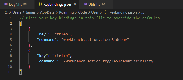
However, Visual Studio isn't as flexible as Vim with these remappings. For example, despite my best efforts, I couldn't find a way to remap the keys for switching between tabs. And this was frustrating, since, as I said before, I would prefer a system where I have a combo to go one tab left and one tab right. With VS Code's system, I find there's a lot of inadvertent jumping around that I find unintuitive compared to other systems like Vim.

Extensions

Now, just as Vim has "plugins" to help you add some new, custom functionality to the editor, VS Code has "extensions" that do the same thing. The first thing I did for VS Code (and that I do for any commercial editor) was to install a Vim extension so that I can use the Vim movement keys even in the graphical editor!

VS Code has a large ecosystem of these, and they are quite easy to install - usually just the click of a button, perhaps combined with restarting the editor.

Pretty much all of the Haskell specific functionality we want also comes through an extension. I use this extension just called "Haskell", which works in conjunction with the Haskell Language Server we also used to support Vim. We'll explore its functionality below.

Incidentally, there was another extension that was crucial for my setup of running on Windows Subsystem for Linux. Visual Studio's way of supporting this is actually through SSH. So you need this special Remote WSL extension.

Language Specific Features

Now let's see the Haskell extension in action. As in Vim, we get notified of compile errors:

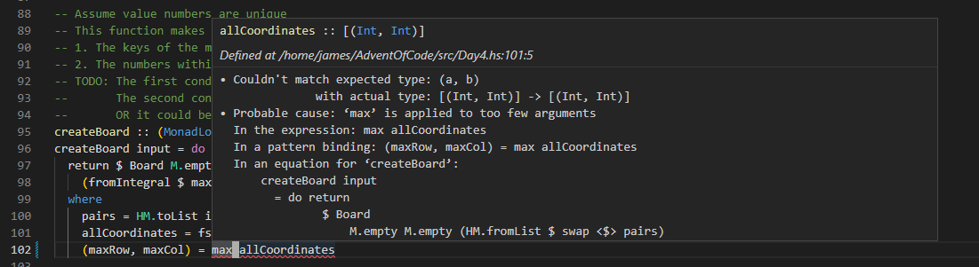
And we also get squiggly lines to indicate lint suggestions. I like the blue highlighting much better than the yellow text from Vim..

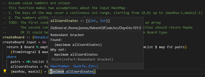
You can also get library suggestions like in Vim, but this time the documentation doesn't appear.

By far the biggest win with Visual Studio is that the extension can autocorrect certain issues, especially missing imports. When you use a new function that it can find in your project or a library, it will bring up this menu and let you fix it with "Ctrl+.". This helps so much with maintaining development flow and now having to scroll back to the top to add the import yourself. It's probably my favorite aspect of using VS Code.

A final area where Visual Studio could offer improvements is with its build systems. It's possible to configure VS to have "Build" and "Test" processes that you can run with assigned keyboard shortcuts. However, I couldn't get these to work with WSL. You have to assign a "stack" executable path. But I think with VS operating in Windows, it rejects the linux version of this file. So I couldn't get those features working. But they might still be possible, especially on Mac.

Conclusions

So all in all, Visual Studio has some nice conveniences. Installing plugins is a bit easier, and the quick correction of issues like imports is very nice. But it's not as customizable as Vim, especially with keyboard shortcuts.

Additionally, since it's a commercial product, Microsoft collects various usage data whenever you use Visual Studio. Certain users might not like this and prefer open source programs as a result. There's a free version of VS called VSCodium, but it lacks most of the useful extensions and is harder to install and use.

And of course there are many other editors out there with viable Haskell extensions, most notably emacs. But I'll leave those for another day.

Make sure to subscribe to stay up to date with all the latest on Monday Morning Haskell! This will give you access to our Subscriber Resources, like our Beginners Checklist!

Using Haskell in Vim: The Basics

Last week I went over some of the basic principles of a good IDE setup. Now in this article and the next, we're going to do this for Haskell in a couple different environments.

A vital component of almost any Haskell setup (at least the two we'll look at) is getting Haskell Language Server running and being able to switch your global GHC version. We covered all that in the last article with GHCup.

In this article we'll look at creating a Haskell environment in Vim. We'll cover how Vim allows us to perform all the basic actions we want, and then we'll add some of the extra Haskell features we can get from using HLS in conjunction with a plugin.

One thing I want to say up front, because I know how frustrating it can be to try repeating something from an article and have it not work: this is not an exhaustive tutorial for installing Haskell in Vim. I plan to do a video on that later. There might be extra installation details I'm forgetting in this article, and I've only tried this on Windows Subsystem for Linux. So hopefully in the future I'll have time to try this out on more systems and have a more detailed look at the requirements.

Base Features

But, for now, let's start checking off the various boxes from last week's list. We had an original list of 7 items for basic functionality. Here are five of them:

1. Open a file in a tab
2. Switch between tabs
3. Open files side-by-side (and switch between them)
4. Open up a terminal to run commands
5. Switch between the terminal and file to edit

Now Vim is a textual editor, meant to be run from a command prompt or terminal. Thus you can't really use the mouse at all in Vim! This is disorienting at first, but it means that all of these actions we have to take must have keyboard commands. Once you learn all these, your coding will get much faster!

To open a new file in a tab, we would use :tabnew followed by the file name (and we can use autocomplete to get the right file). We can then flip between tabs with the commands :tabn (tab-next) and :tabp (tab-previous).

To see multiple files at the same time, we can use the :split command, followed by the file name. This gives a horizontal split. My preference is for a vertical split, which is achieved with :vs and the file name. Instead of switching between files with :tabn and :tabp, we use the command Ctrl+W to go back and forth.

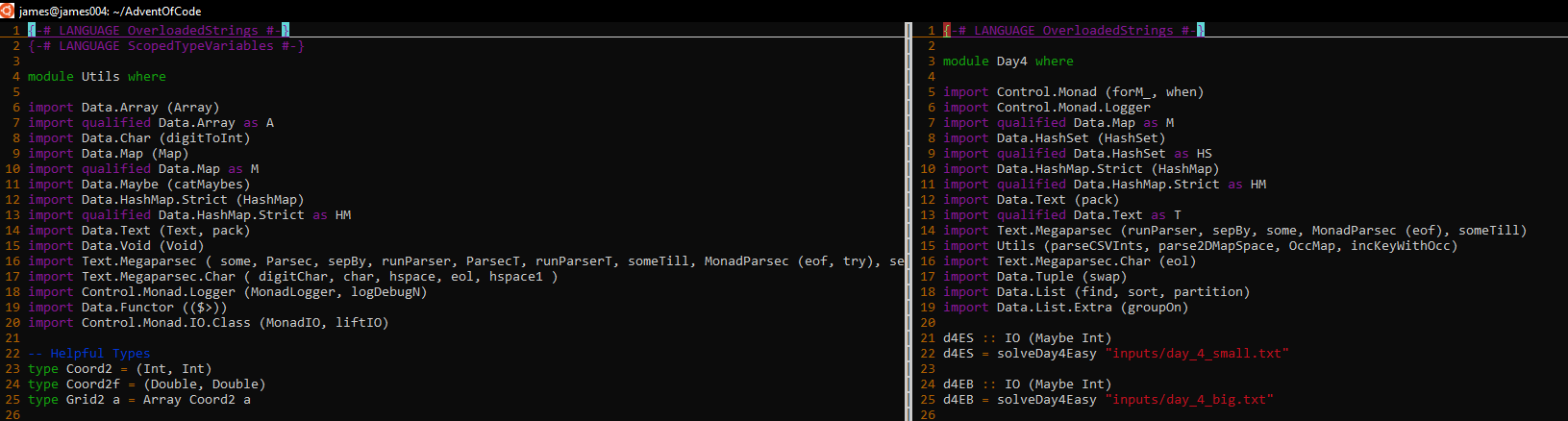
Finally, we can open a terminal using the :term command. By default, this puts the terminal at the bottom of the screen:

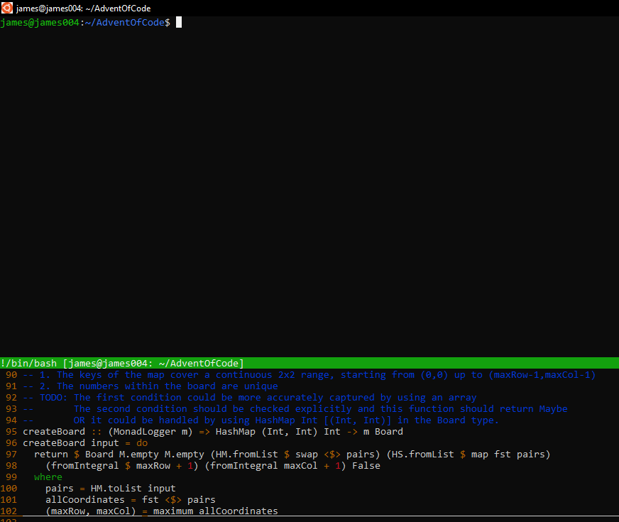
We can also get a side-by-side terminal with :vert term.

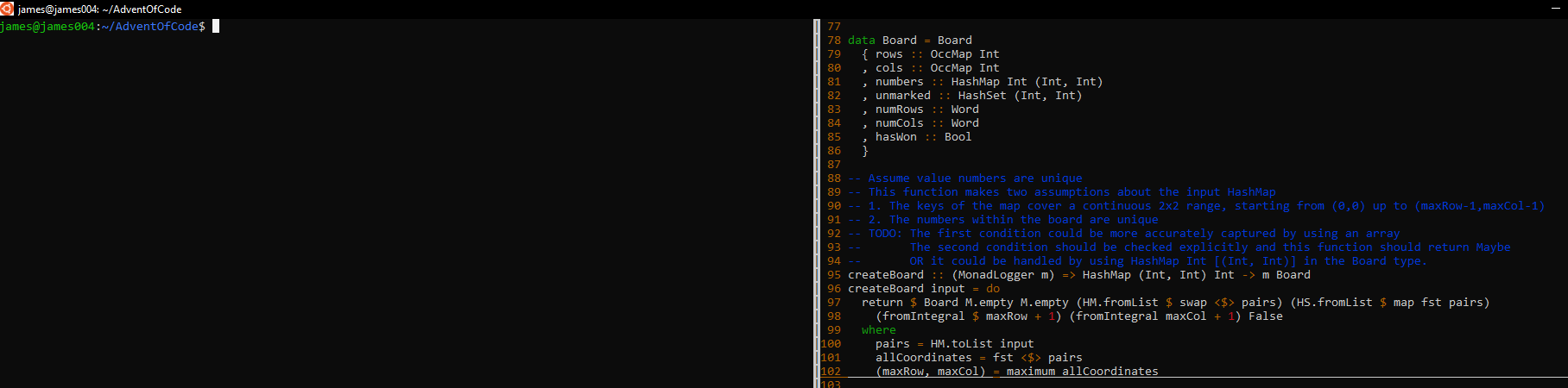
Switching between terminals is the same as switching between split screens: Ctrl+WW.

And of course, obviously, Vim has "Vim movement" keys so you can move around the file very quickly!

Sidebar Support

Now the two other items on the list are related to having a sidebar, another useful base feature in your IDE.

1. Open & close a navigation sidebar
2. Use sidebar to open files

We saw above that it's possible to open new files. But on larger projects, you can't keep the whole project tree in your head, so you'll probably need a graphical reference to help you.

Vim doesn't support such a layout natively. But with Vim (and pretty much every editor), there is a rich ecosystem of plugins and extensions to help improve the experience.

In fact, with Vim, there are multiple ways of installing plugins. The one I ended up deciding on is Vim Plug. I used it to install a Plugin called NerdTree, which gives a nice sidebar view where I can scroll around and open files.

In general, to make a modification to your Vim settings, you modify a file in your home directory called .vimrc. To use NerdTree (after installing Vim Plug), I just added the following lines to that file.

call plug#begin('~/.vim/plugged")
Plug 'preservim/nerdtree'
call plug#end()

Here's what it looks like:

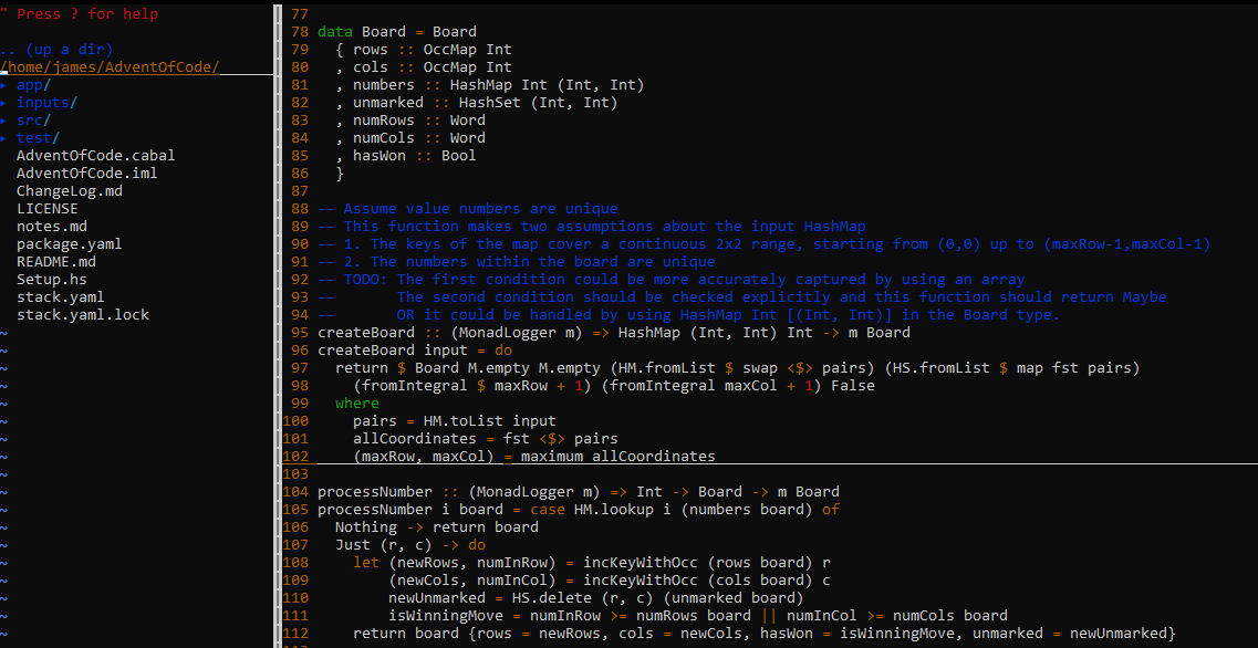
All that's needed to bring this menu up is the command :NERDTree. Switching focus remains the same with Ctrl+WW and so does closing the tab with :q.

Configurable Commands

Another key factor with IDEs is being able to remap commands for your own convenience. I found some of Vim's default commands a bit cumbersome. For example, switching tabs is a common enough task that I wanted to make it really fast. I wanted to do the same with opening the terminal, while also doing so with a vertical split instead of the default horizontal split. Finally, I wanted a shorter command to open the NerdTree sidebar.

By putting the following commands in my .vimrc file, I can get these remappings:

nnoremap <Leader>q :tabp<CR>
nnoremap <Leader>r :tabn<CR>
nnoremap <Leader>t :vert term<CR>
nnoremap <Leader>n :NERDTree<CR>

In these statements, <Leader> refers to a special key that is backslash (\) by default, but also customizable. So now I can switch tabs using \q and \r, open the terminal with \t, and open the sidebar with \n.

Language Specific Features

Now the last (and possibly most important) aspect of setting up the IDE is to get the language-specific features working. Luckily, from the earlier article, we already have the Haskell Language Server running thanks to GHCup. Let's see how to apply this with Vim.

First, we need another Vim plugin to work with the language server. This plugin is called "CoC", and we can install it by including this line in our .Vimrc in the plugins section:

call plug#begin('~/.vim/plugged')
...
Plug 'neoclide/coc.nvim', {'branch': 'release'}
call plug#end()

After installing the plugin (re-open .vimrc or :source the file), we then have to configure the plugin to use the Haskell Language Server. To do this, we have to use the :CocConfig command within Vim, and then add the following lines to the file:

{
  "languageserver": {
    "haskell": {
      "command": "haskell-language-server-wrapper",
      "args": ["--lsp"],
      "rootPatterns": ["*.cabal", "stack.yaml", "cabal.project", "package.yaml", "hie.yaml"],
      "filetypes": ["haskell", "lhaskell"]
    }
  }
}

Next, we have to use GHCup to make sure the "global" version of GHC matches our project's version. So, as an example, we can examine the stack.yaml file and find the resolver:

resolver:
  url: https://raw.githubusercontent.com/commercialhaskell/stackage-snapshots/master/lts/19/13.yaml

The 19.13 resolver corresponds to GHC 9.0.2, so let's go ahead and set that using GHCup:

>> ghcup set ghc 9.0.2

And now we just open our project file and we can start seeing Haskell tips! Here's an example showing a compilation error:

The ability to get autocomplete suggestions from library functions works as well:

And we can also get a lint suggestion (I wish it weren't so "yellow"):

Note that in order for this to work, you must open your file from the project root where the .cabal file is. Otherwise HLS will not work correctly!

# This works!
>> cd MyProject
>> vim src/MyCode.hs

# This does not work!
>> cd MyProject/src
>> vim MyCode.hs

Conclusion

That's all for our Haskell Vim setup! Even though this isn't a full tutorial, hopefully this gives you enough ideas that you can experiment with Haskell in Vim for yourself! Next time, we'll look at getting Haskell working in Visual Studio!

If you want to keep up to date with all the latest on Monday Morning Haskell, make sure to subscribe to our mailing list! This will also give you access to our subscriber resources, including beginner friendly resources like our Beginners Checklist!

Using GHCup!

When it comes to starting out with Haskell, I usually recommend installing Stack. Stack is an effective one-stop shop. It automatically installs Cabal for you, and it's also able to install the right version of GHC for your project. It installs GHC to a sandboxed location, so you can easily use different versions of GHC for different projects.

But there's another good program that can help with these needs! This program is called GHCup ("GHC up"). It fills a slightly different role from Stack, and it actually allows more flexibility in certain areas. Let's see how it works!

How do I install GHCup?

Just like Stack, you can install GHCup with a single terminal command. Per the documentation, you can use this command on Linux, Mac, and Windows Subsystem for Linux:

curl --proto '=https' --tlsv1.2 -sSf https://get-ghcup.haskell.org | sh

See the link above for special instructions on a pure Windows setup.

What does GHCup do?

GHCup can handle the installation of all the important programs that make Haskell work. This includes, of course, the compiler GHC, Cabal, and Stack itself. What makes it special is that it can rapidly toggle between the different versions of all these programs, which can give you more flexibility.

Once you install GHCup, this should install the recommended version of each of these. You can see what is installed with the command ghcup list.

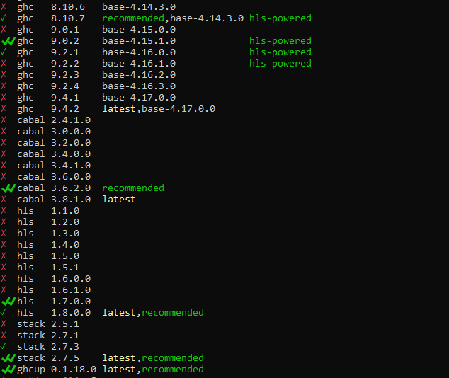
The "currently installed" version of each has a double checkmark as you can see in the picture. When you use each of these commands with the --version argument, you should see the version indicated by GHCup:

>> stack --version
Version 2.7.5
>> cabal --version
cabal-install version 3.6.2.0
>> ghc --version
The Glorious Glasgow Haskell Compilation System, version 9.02

How do I switch versions with GHCup?

Any entry with a single green checkmark is "installed" on your system but not "set". You can set it as the "global" version with the ghcup set command.

>> ghcup set ghc 8.10.7
[ Info ] GHC 8.10.7 successfully set as default version
>> ghc --version
The Glorious Glasgow Haskell Compilation System, version 8.10.7

Versions with a red x aren't installed but are available to download. If a version isn't installed on your system, you can use ghcup install to get it:

>> ghcup install stack 2.7.1

Then you need to set the version to use it:

>> ghcup set stack 2.7.1
>> stack --version
Version 2.7.1

Note that the specific example with Stack might not work if you originally installed Stack through its own installer before using GHCup.

GHCup User Interface

On most platforms, you can also use the command: ghcup tui. This brings up a textual user interface that allows you to make these changes quickly! It will bring up a screen like this on your terminal, allowing you to use the arrow keys to set the versions as you desire.

All the commands are on screen, so it's very easy to use!

Notes on Stack and GHC

An important note on setting the "global" version of GHC is that this does not affect stack sandboxing. Even if you run ghcup set ghc 8.10.7, this won't cause any problems for a stack project using GHC 9.02. It will build as normal using 9.02.

So why does it even matter what the global version of GHC is? Let's find out!

GHCup and IDEs

Why do I mention GHCup when my last article was talking about IDEs? Well the one other utility you can install and customize with GHCup is the Haskell Language Server, which shows up in the GHCup output as the program hls. This is a special program that enables partial compilation, lint suggestions and library autocompletion within your IDE (among other useful features). As we'll explore in the next couple articles, Haskell Language Server can be a little tricky to use!

Even though Stack uses sandboxed GHC versions, HLS depends on the "global" version of GHC. And changing the "global" version to a particular version you've installed with stack is a little tricky if you aren't super familiar with Haskell's internals and also comfortable with the command line. So GHCup handles this smoothly.

Imagine we have two projects with different Stack resolvers (and in this case different GHC versions).

# stack.yaml #1
# (GHC 9.0.2)
resolver:
  url: https://raw.githubusercontent.com/commercialhaskell/stackage-snapshots/master/lts/19.16

# stack.yaml #2
# (GHC 8.10.7)
resolver:
  url: https://raw.githubusercontent.com/commercialhaskell/stackage-snapshots/master/lts/18.26

If we want to get code suggestions in our first project, we just need to run this command before open it in the editor:

ghcup set ghc 9.0.2

And if we then want to switch to our second project, we just need one command to get our hints again!

ghcup set ghc 8.10.7

And of course, in addition to switching the GHC version, GHCup installs HLS for you and allows you to switch its version to keep up with updates.

Conclusion

With a basic understanding of HLS and switching GHC versions, we're now in a good position to start designing a really strong Haskell IDE! In the next couple of articles, we'll see a couple examples of this!

Keep up to date with all the latest news on Monday Morning Haskell by subscribing to our mailing list! This will also give you access to our subscriber resources!

What Makes a Good IDE?

Sometimes in the past I've read articles about people's IDE setups and thought "wow, they spend way too much time thinking about this." Now maybe sometimes people do go overboard. But on the other hand, I think it's fair to say I've been neglecting the importance of my development environment in my own practice.

A quick look at some of my videos in the last couple years can show you this fact. This whole playlist is a good example. I'm generally working directly with Vim with virtually no language features beyond syntax highlighting. I think my environment even lacked any semblance of auto-completion, so if I wasn't copying something directly, I would be writing the whole thing out.

If I wanted to compile or run my code, I would switch to a terminal opened in a separate window and manually enter commands. At the very least, I could switch between these terminals pretty easily. But opening new files and trying to compare files side-by-side was a big pain.

So after reflecting on these experiences, one of my resolutions this year has been to improve my Haskell development environment. In this first article on the subject, I'll consider the specific elements of what makes a good IDE and how we can use a systematic approach to build our ideal environment.

Listing Our Needs

Designing a good environment requires us to be intentional. This means thinking carefully about what we're using our environment for, and getting into the details of the specific actions we want.

So a good starting point is to list out the important actions we want to take within our editor. Here's my preliminary list:

1. Open a file in a tab
2. Switch between tabs
3. Open files side-by-side (and switch between them)
4. Open & close a navigation sidebar
5. Use sidebar to open files
6. Open up a terminal to run commands
7. Switch between the terminal and file to edit

But having these features available is just the start. We also want to do things quickly!

Moving Fast

I used to play Starcraft for a few years. And while I wasn't that good, I was good enough to learn one important lesson to apply to programming. The keyboard is way more efficient than the mouse. The mouse gives the advantage of moving in 2D space. But overall the keyboard is much faster and more precise. So in your development environment, it's very important to learn to do as many things as possible with keyboard shortcuts.

So as a practical matter, I recommend thinking carefully about how you can accomplish your most common tasks (like the features we listed above) with the keyboard. Write these down if you have to!

It helps a lot if you use an editor that allows you to remap keyboard commands. This will give you much more control over how your system works and let you pick key-bindings that are more intuitive for you. Programs like Vim and Emacs allow extensive remapping and overall customization. However, More commercial IDEs like Visual Studio and IntelliJ will still usually allow you some degree of customization.

Speaking of Vim and Emacs, the general movement keys each has (for browsing through and editing your file) are extremely useful for helping improve your general programming speed. Most IDEs have plugins that allow you to incorporate these movement keys.

The faster you're able to move, the more programming will feel like an enjoyable experience, almost like a game! So you should really push yourself to learn these keyboard shortcuts instead of resorting to using the mouse, which might be more familiar at first. In a particular programming session, try to see how long you can go without using the mouse at all!

Language Features

The above features are useful no matter what language or platform you're using. Many of them could be described as "text editor" features, rather than features of a "development environment". But there are also specific things you'll want for the language you're working with.

Syntax highlighting is an essential feature, and autocomplete is extremely important. Basic autocomplete works with the files you have open, but more advanced autocomplete can also use suggestions from library functions.

At the next level of language features, we would want syntax hints, lint suggestions and partial compilation to suggest when we have errors (for compiled languages). These also provide major boosts to your productivity. You can correct errors on the fly, rather than trying to determine the right frequency to switch to your terminal, try compiling your code, and match up the errors with the relevant area of code.

One final area of improvement you could have is integrated build and test commands. Many commercial IDEs have these for particular language setups. But it can be a bit trickier to make these work for Haskell. This is why I still generally rely on opening a terminal instead of using such integrations.

Conclusion

In the next couple articles, I'll go through a few different options I've considered and experimented with for my Haskell development setup. I'll list a few pros and cons of each and give a few tips on starting out with them. I'll also go through a couple tools that are generally useful to making many development environments work with Haskell.

To make sure you're up to date on all our latest news, make sure you've subscribed to our mailing list! This will give you access to all our subscriber resources, including our Beginners Checklist!

Haskell for High Schoolers: Paradigm Conference!

Here's a quick announcement today, aimed at those younger Haskellers out there. If you're in middle school or high school (roughly age 18 and below), you should consider signing up for Paradigm Conference this coming weekend (September 23-25)! This is a virtual event aimed at teaching younger students about functional programming.

The first day of the conference consists of a Hackathon where you'll get the chance to work in teams to solve a series of programming problems. I've been emphasizing this sort of problem solving a lot in my streaming sessions, so I think it will be a great experience for attendees!

On the second day, there will be some additional coding activities, as well as workshops and talks from speakers, including yours truly. Since I'll be offline the whole weekend, my talk will be pre-recorded, but it will connect a lot of the work I've been doing in the last couple of months with respect to Data Structures and Dijkstra's algorithm. So if you've enjoyed those series independently, you might enjoy the connections I try to make between these ideas. This video talk will include a special offer for Haskell newcomers!

So to sign up and learn more, head over to the conference site, and start getting ready!

Everyday Applicatives!

I recently revised the Applicatives page on this site, and it got me wondering...when do I use applicatives in my code? Functors are simpler, and monads are more ubiquitous. But applicatives fill kind of an in-between role where I often don't think of them too much.

But a couple weeks ago I encountered one of those small coding problems in my day job that's easy enough to solve, but difficult to solve elegantly. And as someone who works with Haskell, of course I like to make my code as elegant as possible.

But since my day job is in C++, I couldn't find a good solution. I was thinking to myself the whole time, "there's definitely a better solution for this in Haskell". And it turns out I was right! And the answer in this case, was to functions specific to Applicative!

To learn more about applicative functors and other functional structures, make sure to read our Monads series! But for now, let's explore this problem!.

Setup

So at the most basic level, let's imagine we're dealing with a Messsage type that has a timestamp:

class Message {
  Time timestamp;
  ...
}

We'd like to compare two messages based on their timestamps, to see which one is closer to a third timestamp. But to start, our messages are wrapped in a StatusOr object for handling errors. (This is similar to Either in Haskell).

void function() {
  ...
  Time baseTime = ...;
  StatusOr<Message> message1 = ...;
  StatusOr<Message> message2 = ...;
}

I now needed to encode this logic:

1. If only one message is valid, do some logic with that message
2. If both messages are valid, pick the closer message to the baseTime and perform the logic.
3. If neither message is valid, do a separate branch of logic.

The C++ Solution

So to flesh things out more, I wrote a separate function signature:

void function() {
  ...
  Time baseTime = ...;
  StatusOr<Message> message1 = ...;
  StatusOr<Message> message2 = ...;
  optional<Message> closerMessage = findCloserMessage(baseTime, message1, message2);
  if (closerMessage.has_value()) {
    // Do logic with "closer" message
  } else {
    // Neither is valid
  }
}

std::optional<Message> findCloserMessage(
    Time baseTime,
    const StatusOr<Message>& message1,
    const StatusOr<Message>& message2) {
     ...
}

So the question now is how to fill in this helper function. And it's simple enough if you embrace some branches:

std::optional<Message> findCloserMessage(
    Time baseTime,
    StatusOr<Message> message1,
    StatusOr<Message> message2) {
    if (message1.isOk()) {
        if (message2.isOk()) {
            if (abs(message1.value().timestamp - baseTime) < abs(message2.value().timestamp - baseTime)) {
                return {message1.value()};
            } else {
                return {message2.value()};
            }
        } else {
            return {message1.value()};
        }
    } else {
        if (message2.isOk()) {
            return {message2.value()};
        } else {
            return std::nullopt;
        }
    }
}

Now technically I could combine conditions a bit in the "both valid" case and save myself a level of branching there. But aside from that nothing else really stood out to me for making this better. It feels like we're doing a lot of validity checks and unwrapping with .value()...more than we should really need.

The Haskell Solution

Now with Haskell, we can actually improve on this conceptually, because Haskell's functional structures give us better ways to deal with validity checks and unwrapping. So let's start with some basics.

data Message = Message
  { timestamp :: UTCTime
  ...
  }

function :: IO ()
function = do
  let (baseTime :: UTCTime) = ...
  (message1 :: Either IOError Message) <- ...
  (message2 :: EIther IOError Message) <- ...
  let closerMessage' = findCloserMessage baseTime message1 message2
  case closerMessage' of
    Just closerMessage -> ...
    Nothing -> ...

findCloserMessage ::
  UTCTime -> Either IOError Message -> Either IOError Message -> Maybe Message
findCloserMessage baseTime message1 message2 = ...

How should we go about implementing findCloserMessage?

The answer is in the applicative nature of Either! We can start by defining a function that operates directly on the messages and determines which one is closer to the base:

findCloserMessage baseTime message1 message2 = ...
  where
    f :: Message -> Message -> Message
    f m1@(Message t1) m2@(Message t2) =
      if abs (diffUTCTime t1 baseTime) < abs (diffUTCTime t2 basetime)
        then m1 else m2

We can now use the applicative operator <*> to apply this operation across our Either values. The result of this will be a new Either value.

findCloserMessage baseTime message1 message2 = ...
  where
    f :: Message -> Message -> Message
    f m1@(Message t1) m2@(Message t2) =
      if abs (diffUTCTime t1 baseTime) < abs (diffUTCTime t2 basetime)
        then m1 else m2

    bothValidResult :: Either IOError Message
    bothValidResult = pure f <*> message1 <*> message2

So if both are valid, this will be our result. But if either of our inputs has an error, we'll get this error as the result instead. What happens in this case?

Well now we can use the Alternative behavior of many applicative functors such as Either. This lets us use the <|> operator to combine Either values so that instead of getting the first error, we'll get the first success. So we'll combine our "closer" message if both are valid with the original messages:

import Control.Applicative

findCloserMessage baseTime message1 message2 = ...
  where
    f :: Message -> Message -> Message
    f m1@(Message t1) m2@(Message t2) =
      if abs (diffUTCTime t1 baseTime) < abs (diffUTCTime t2 basetime)
        then m1 else m2

    bothValidResult :: Either IOError Message
    bothValidResult = pure f <*> message1 <*> message2

    allResult :: Either IOError Message
    allResult = bothValidResult <|> message1 <|> message2

The last step is to turn this final result into a Maybe value:

import Control.Applicative
import Data.Either

findCloserMessage ::
  UTCTime -> Either IOError Message -> Either IOError Message -> Maybe Message
findCloserMessage baseTime message1 message2 =
  if isRight allResult then Just (fromRight allResult) else Nothing
  where
    f :: Message -> Message -> Message
    f m1@(Message t1) m2@(Message t2) =
      if abs (diffUTCTime t1 baseTime) < abs (diffUTCTime t2 basetime)
        then m1 else m2

    bothValidResult :: Either IOError Message
    bothValidResult = pure f <*> message1 <*> message2

    allResult :: Either IOError Message
    allResult = bothValidResult <|> message1 <|> message2

The vital parts of this are just the last 4 lines. We use applicative and alternative operators to simplify the logic that leads to all the validity checks and conditional branching in C++.

Conclusion

Is the Haskell approach better than the C++ approach? Up to you! It feels more elegant to me, but maybe isn't as intuitive for someone else to read. We have to remember that programming isn't a "write-only" activity! But these examples are still fairly straightforward, so I think the tradeoff would be worth it.

Now is it possible to do this sort of refactoring in C++? Possibly. I'm not deeply familiar with the library functions that are possible with StatusOr, but it certainly wouldn't be as idiomatic.

If you enjoyed this article, make sure to subscribe to our monthly newsletter! You should also check out our series on Monads and Functional Structures so you can learn more of these tricks!

My New Favorite Monad?

In my last article, I introduced a more complicated example of a problem using Dijkstra's algorithm and suggested MonadLogger as an approach to help debug some of the intricate helper functions.

But as I've started getting back to working on some of the "Advent of Code" type problems, I've come to the conclusion that this kind of logging might be more important than I initially realized. At the very least, it's gotten me thinking about improving my general problem solving process. Let's explore why.

Hitting a Wall

Here's an experience I've had quite a few times, especially with Haskell. I'll be solving a problem, working through the ideas in my head and writing out code that seems to fit. And by using Haskell, a lot of problems will be resolved just from making the types work out.

And then, ultimately, the solution is wrong. I don't get the answer I expected, even though everything seems correct.

So how do I fix this problem? A lot of times (unfortunately), I just look at the code, think about it some more, and eventually realize an idea I missed in one of my functions. This is what I would call an insight-based approach to debugging.

Insight is a useful thing. But used on its own, it's probably one of the worst ways to debug code. Why do I say this? Because insight is not systematic. You have no process or guarantee that you'll eventually come to the right solution.

So what are systematic approaches you can take?

Systematic Approaches to Debugging

Three general approaches come to my mind when I think about systematic debugging methods.

1. Writing unit tests
2. Using a debugging program (e.g. GDB)
3. Using log statements

Unit Tests

The first approach is distinct from the other two in that it is a "black box" method. With unit tests, we provide a function with particular inputs and see if it produces the outputs we expect. We don't need to think about the specific implementation of the function in order to come up with these input/output pairs.

This approach has advantages. Most importantly, when we write unit tests, we will have an automated program that we can always run to verify that the function still behaves how we expect. So we can always refactor our function or try to improve its performance and still know that it's giving us the correct outputs.

Writing unit tests proactively (test driven development) can also force us to think about edge cases before we start programming, which will help us implement our function with these cases in mind.

However, unit testing has a few disadvantages as well. Sometimes it can be cumbersome to construct the inputs to unit-test intermediate functions. And sometimes it can be hard to develop non-trivial test cases that really exercise our code at scale, because we can't necessarily know the answer to harder cases beforehand. And sometimes, coming up with a unit test that will really find a good edge case takes the same kind of non-systematic insight that we were trying to avoid in the first place.

Unit tests can be tricky and time-consuming to do well, but for industry projects you should expect to unit test everything you can. So it's a good habit to get into.

Using a Debugger

The second approach on the list is more of a "white box" approach. Debuggers allow us to explore the interior state of our function while it is running and see if the values match our expectations.

So for example, the typical debugger can set a breakpoint so that the program pauses execution in the middle of our function. We can then explore all the values in scope at this point. And examining these values can tell us if the assumptions we're making about our code are correct. We can then step the program forward and see if these values update the way we expect.

However, it is a bit harder to use debugging programs with Haskell. With most imperative languages, the ordering of the machine code (at least when unoptimized) somewhat resembles the order of the code you write in the editor. But Haskell is not an imperative language, so the ordering of operations is more complicated. This is made even worse because of Haskell's laziness.

But debuggers are still worth pursuing! I'll be exploring this subject more in the future. For now, let's move on to our last approach.

Log Messages

What are the advantages of using a logging approach? Are "print statements" really the way to go?

Well this is the quickest and easiest way to get some information about your program. Anyone who's done a technical interview knows this. When something isn't going right in that kind of fast-paced situation, you don't have time to write unit tests. And attaching a debugger isn't an option in interview environments like coderpad. So throwing a quick print statement in your code can help you get "unstuck" without spending too much time.

But generally speaking, you don't want your program to be printing out random values. Once you've resolved your issue, you'll often get rid of the debugging statements. Since these statements won't become part of your production code, they won't remain as a way to help others understand and debug your code, as unit tests do.

Logging and Frustration in Haskell

Considering these three different methods, logging and print statements are the most common method for anyone who is first learning a language. Setting up a debugger can be a complex task that no beginner wants to go through. Nor does a novice typically want to spend the time to learn unit test frameworks just so they can solve basic problems.

This presents us with a conundrum in helping people to learn Haskell. Because logging is not intuitive in Haskell. Or rather, proper logging is not intuitive.

Showing someone the main :: IO () and then using functions like print and putStrLn is easy enough. But once beginners start writing "pure" functions to solve problems, they'll get confused about how to use logging statements, since the whole point of pure functions is that we can't just add print statements to them.

There are, of course, "unsafe" ways to do this with the trace library and unsafePerformIO. But even these options use patterns that are unintuitive for beginners to the language.

Start with Logger Monad

With these considerations, I'm going to start an experiment for a while. As I write solutions to puzzle problems (the current focus of my Haskell activity), I'm going to write all my code with a MonadLogger constraint. And I would consider the idea of recommending a beginner to do the same. My hypothesis is that I'll solve problems much more quickly with some systematic approach rather than unsystematic insight-driven-development. So I want to see how this will go.

Using MonadLogger is much more "pure" than using IO everywhere. While the most common instances of the logger monad will use IO, it still has major advantages over just using the IO monad from a "purity" standpoint. The logging can be disabled. You can also put different levels of logging into your program. So you can actually use logging statements to log a full trace of your program, but restrict it so that the most verbose statements are at DEBUG and INFO levels. In production, you would disable those messages so that you only see ERROR and WARN messages.

Most importantly, you can't do arbitrary IO activity with just a MonadLogger constraint. You can't open files or send network requests.

Of course, the price of this approach for a beginner is that the newcomer would have to get comfortable with having monadic code with a typeclass constraint before they necessarily understand these topics. But I'm not sure that's worse than using IO everywhere. And if it relieves the frustration of "I can't inspect my program", then I think it could be worthwhile for someone starting out with Haskell.

Conclusion

If you want to see me using this approach on real problems, then tune into my Twitch Stream! I usually stream 5 times a week for short periods. Some of these episodes will end up on my YouTube channel as well.

Meanwhile, you can also subscribe to the mailing list for more updates! This will give you access to Monday Morning Haskell's subscriber resources!

Dijkstra with Monads!

Last time on the blog, we considered this library version of Dijkstra's algorithm that you can find on Hackage.

dijkstra ::
    (Foldable f, Num cost, Ord cost, Ord State)
  => (state -> f state) -- Function to generate list of neighbors
  -> (state -> state -> cost) -- Function for cost generation
  -> (state -> Bool) -- Destination predicate
  -> state -- Initial state
  -> Maybe (cost, [state]) -- Solution cost and path, Nothing if goal is unreachable

However, there are a number of situations where this might be insufficient. In this article we'll consider some reasons why you would want to introduce monads into your solution for Dijkstra's algorithm. Let's explore some of these reasons!

Note! This is a "coding ideas" blog, rather than an "In Depth Tutorial" blog (see this article for a summary of different reading styles). Some of the code sampled are pretty well fleshed out, but some of them are more hypothetical ideas for you to try out on your own!

The Monadic Version

In addition to the "pure" version of Dijkstra's algorithm, the Algorithm.Search library also provides a "monadic" version. This version allows each of the input functions to act within a monad m, and of course gives its final result within this monad.

dijkstraM ::
    (Monad m, Foldable f, Num cost, Ord cost, Ord State)
  => (state -> m (f state))
  -> (state -> state ->m cost)
  -> (state -> m Bool)
  -> state
  -> m (Maybe (cost, [state]))

Now, if you've read our Monads Series, you'll know that a monad is a computational context. What are the kinds of contexts we might find ourselves in while performing Dijkstra's algorithm? Here are a few ideas to start with.

1. We're reading our graph from a global state (mutable or immutable) 2.Our graph functions require reading a file or making a network call
2. We would like to log the actions taken in our graph.

Let's go through some pseudocode examples to see how each of these could be useful.

Using a Global State

A global mutable state is represented with (of course) the State monad. An immutable global state uses the Reader monad to represent this context. Now, taken in a simple way, the Reader context could allow us to "pass the graph" without actually including it as an argument:

import qualified Data.Array as A
import Control.Monad.Reader
import Algorithm.Search (dijkstraM)

newtype Graph2D = Graph2D (A.Array (Int, Int) Int)

getNeighbors :: A.Array (Int, Int) Int -> (Int, Int) -> [(Int, Int)]

findShortestPath :: Graph2D -> (Int, Int) -> (Int, Int) -> Maybe (Int, [(Int, Int)])
findShortestPath graph start end = runReader
  (dijkstraM neighbors cost (return . (== end)) start)
  graph
  where
    cost :: (Int, Int) -> (Int, Int) -> Reader Graph2D Int
    cost _ b = do
      (Graph2D gr) <- ask
      return $ gr A.! b

    neighbors :: (Int, Int) -> Reader Graph2D [(Int, Int)]
    neighbors source = do
      (Graph2D gr) <- ask
      return $ getNeighbors gr source

If we're already in this monad for whatever reason, then this could make sense. But on its own, it's not necessarily much of an improvement over partial function application.

A mutable state could be useful in certain circumstances as well. We likely wouldn't want to mutate the graph itself during iteration, as this would invalidate the algorithm. However, we could store certain metadata about what is happening during the search. For instance, we might want to track how often certain nodes are returned as a potential neighbor.

import qualified Data.HashMap.Strict as HM
import Control.Monad.State
import Data.Maybe (fromMaybe)
import Data.Foldable (find)

newtype Graph = Graph
   { edges :: HM.HashMap String [(String, Int)] }

type Metadata = HM.HashMap String Int
incrementKey :: String -> Metadata -> Metadata
incrementKey k metadata = HM.insert k (count + 1) metadata
  where
    count = fromMaybe 0 (HM.lookup k metadata)

findShortestPath :: Graph -> String -> String -> Maybe (Int, [String])
findShortestPath graph start end = evalState
  (dijkstraM neighbors cost (return . (== end)) start)
  HM.empty
  where
    cost :: String -> String -> State Metadata Int
    cost n1 n2 = 
      let assocs = fromMaybe [] (HM.lookup n1 (edges graph))
          costForN2 = find (\(n, _) -> n == n2) assocs
      in  case costForN2 of
            Nothing -> return maxBound
            Just (_, x) -> return x
    neighbors :: String -> State Metadata [String]
    neighbors node = do
      let neighbors = fst <$> fromMaybe [] (HM.lookup node (edges graph))
      metadata <- get
      put $ foldr incrementKey metadata neighbors
      return neighbors

In this implementation, we end up discarding our metadata, but if we wanted to we could include it as an additional output to help us understand what's happening in our search.

Reading from Files

In many cases, our "graph" is actually too big to fit within memory. In various cases, the entire graph could be distributed across many files on our system. Consider this simplified example:

data Location = Location
  { filename :: FilePath
  , tag :: String
  ...
  }

Each file could track a certain "region" of your map, with references to certain locations "on the edge" whose primary data must be found in a different file. This means you'll need to have access to the file system to ensure you can find all the "neighbors" of a particular location: This means you'll need the IO monad in Haskell!

getMapNeighbors :: Location -> IO [Location]
-- Open original locations file
-- Find tag and include neighboring tags together with references to other files

This matches the signature of the "neighbor generator" function in dijkstraM, so we'll be able to pass this function as the first argument.

Using Network Calls

Here's a fun example. Consider wiki-racing - finding the shortest path between the Wikipedia pages of two topics using only the links in the bodies of those pages. You could (theoretically) write a program to do this for you. You might create a type like this:

data WikiPage = WikiPage
  { pageTitle :: Text
  , url :: URL
  , bodyContentHtml :: Text
  }

In order to find the "neighbors" of this page, you would first have to parse the body HTML and find all the wikipedia links within it. This could be done in a pure fashion. But in order to create the WikiPage objects for each of those links, you would then need to send an HTML GET request to get their body HTML. Such a network call would require the IO monad (or some other MonadIO), so you're function will necessarily look like:

getWikiNeighbors :: WikiPage -> IO [Wikipage]

But if you successfully implement that function, it's very easy to apply dijkstraM because the "cost" of each hop is always 1!

findShortestWikiPath :: Text -> Text -> IO (Maybe (Int, [WikiPage]))
findShortestWikiPath start end = do
  firstPage <- findWikiPageFromTitle start
  dijkstraM getWikiNeighbors (\_ _ -> return 1) (return . (== end)) firstPage

findWikiPageFromTitle :: Text -> IO WikiPage
...

Of course, because the cost is always 1 this is actually a case where breadth first search would work more simply than Dijkstra's algorithm, so you could use the function bfsM from the same library!

Logging

Another common context for problem solving is the logging context. While we are solving our problem, we might want to record helpful statements telling us what is happening so that we can debug when things are going wrong. This happens using the MonadLogger typeclass, with a few interesting functions we can use, indicating different "levels" of logging.

class MonadLogger m where
  ...

logDebugN :: (MonadLogger m) => Text -> m ()
logInfoN :: (MonadLogger m) => Text -> m ()
logWarnN :: (MonadLogger m) => Text -> m ()
logErrorN :: (MonadLogger m) => Text -> m ()

Now, unlike the previous two examples, this doesn't require the IO monad. A couple of the most common implementations of this monad class will, in fact, use IO functionality (printing to the screen or logging to a file). But this isn't necessary. You can still do logging in a "pure" way by storing the log messages in a sequence or other structure so you can examine them at the end of your program.

When would we want this for Dijkstra's algorithm? Well, sometimes the process of determining neighbors and costs can be complicated! I'll motivate this by introducing a more complicated example of a Dijkstra's algorithm problem.

A Complicated Example

Here's an example from last year's Advent of Code challenge. You can read the full description on that page. This problem demonstrates a less intuitive use of Dijkstra's algorithm.

The problem input is a "map" of sorts, showing a diagram of 4 rooms leading into one shared hallway.

#############
#...........#
###B#C#B#D###
  #A#D#C#A#
  #########

Each of the four rooms is filled with "tokens", which come in 4 different varieties, A, B, C, D. (The Advent of Code description refers to them as "Amphipods", but that takes a while to write out, so I'm simplifying to "tokens").

We want to move the tokens around so that the A tokens end in the far left room, the B tokens in the room next to them, and so on.

#############
#...........#
###A#B#C#D###
  #A#B#C#D#
  #########

But there are rules on how these tokens move. You can only move each token twice. Once to get it into an empty space in the hallway, and once to get it from the hallway to its final room. And tokens can't move "past" each other within the hallway.

Now each token has a specific cost for each space it moves.

A = 1 energy per move
B = 10 energy per move
C = 100 energy per move
D = 1000 energy per move

So you want to move the token's into the final state with the lowest total cost.

Using Dijkstra's Algorithm

It turns out the most efficient solution (especially at a larger scale) is to treat this like a graph problem and use Dijkstra's algorithm! Each "state" of the problem is like a node in our graph, and we can move to certain "neighboring" nodes by moving tokens at a certain cost.

But the implementation turns out to be quite tricky! To give you an idea of this, here are some of the data type names and functions I came up with.

data Token = ...

data HallSpace = ...

data TokenGraphState = ...

tokenEdges :: TokenGraphState -> [(TokenGraphState, Int)]

updateStateWithMoveFromRoom :: Token -> HallSpace -> Int -> TokenGraphState -> (TokenGraphState, Int)

updateStateWithMoveFromHall :: Token -> HallSpace -> Int -> TokenGraphState -> (TokenGraphState, Int)

validMovesToHall :: Token -> TokenGraphState -> [(HallSpace, Int)]

validMoveToRoom :: TokenGraphState -> (HallSpace, TokenGraphState -> Maybe Token) -> Maybe (Int, Token, HallSpace)

And these are just the functions with complex logic! There are even a few more simple helpers beyond this!

But when I ran this implementation, I didn't get the right answer! So how could I learn more about my solution and figure out what's going wrong? Unit testing and applying a formal debugger would be nice, but simply being able to print out what is going on in the problem is a quicker way to get started.

Haskell doesn't let you (safely) print from pure functions like I've written above, nor can you add values to a global logging state. So we can fix this by modifying the type signatures to instead use a MonadLogger constraint.

tokenEdges :: (MonadLogger m) => TokenGraphState -> m [(TokenGraphState, Int)]

updateStateWithMoveFromRoom :: (MonadLogger m) => Token -> HallSpace -> Int -> TokenGraphState -> (TokenGraphState, Int)

updateStateWithMoveFromHall :: (MonadLogger m) => Token -> HallSpace -> Int -> TokenGraphState -> m (TokenGraphState, Int)

validMovesToHall :: (MonadLogger m) => Token -> TokenGraphState -> m [(HallSpace, Int)]

validMoveToRoom :: (MonadLogger m) => TokenGraphState -> (HallSpace, TokenGraphState -> Maybe Token) -> m (Maybe (Int, Token, HallSpace))

Now it's simple enough to modify a function to give us some important information about what's happening. Hopefully this is enough to help us solve the problem.

We would like to limit the number of functions that "need" the monadic action. But in practice, it is frustrating to find you need a monad in a deeper function of your algorithm because you'll need to modify everything on its call stack. So it might be a good idea to add at least a basic monad constraint from the beginner!

(Update: I did a full implementation of this particular problem that incorporates the logger monad!)

Conclusion

Next time on the blog, we'll start talking more generally about this idea of using monads to debug, especially MonadLogger. We'll consider the implementation pattern of "monads first" and different ways to approach this.

Make sure you're staying up to date with the latest news from Monday Morning Haskell by subscribing to our mailing list! This will also give you access to our subscriber resources!

Dijkstra Comparison: Looking at the Library Function

In the last few articles I've gone through my approach for generalizing Dijkstra's algorithm in Haskell. The previous parts of this included:

1. Simple Form of Dijkstra's Algorithm
2. Generalizing with a Multi-Param Typeclass
3. Generalizing with a Type Family
4. A 2D Graph example

But of course I wasn't the first person to think about coming up with a general form of Dijkstra's algorithm in Haskell. Today, we'll look at the API for a library implementation of this algorithm and compare it to the implementations I thought up.

Comparing Types

So let's look at the type signature for the library version of Dijkstra's algorithm.

dijkstra ::
    (Foldable f, Num cost, Ord cost, Ord State)
  => (state -> f state) -- Function to generate list of neighbors
  -> (state -> state -> cost) -- Function for cost generation
  -> (state -> Bool) -- Destination predicate
  -> state -- Initial state
  -> Maybe (cost, [state]) -- Solution cost and path, Nothing if goal is unreachable

We'd like to compare this against the implementations in this series, but it's also useful to think about the second version of this function from the library: dijkstraAssoc. This version combines the functions for generating neighbors and costs:

dijkstraAssoc ::
    (Num cost, Ord cost, Ord state)
  => (state -> [(state, cost)])
  -> (state -> Bool)
  -> state
  -> Maybe (cost, [state])

And now here's the signature for the Multi-Param typeclass version I wrote:

findShortestDistance ::
    (Hashable node, Eq node, Num cost, Ord cost, DijkstraGraph graph)
  => graph -> node -> node -> Distance cost

We can start the comparison by pointing out a few surface-level differences..

First, the library uses Nothing to represent a failure to reach the destination, instead of a Distance type with Infinity. This is a sensible choice to spare API users from incorporating an internal type into their own code. However, it does make some of the internal code more cumbersome.

Second, the library function also includes the full path in its result which is, of course, very helpful most of the time. The implementation details for this aren't too complicated, but it requires tracking an extra structure, so I have omitted it so far in this series.

Third, the library function takes a predicate for its goal, instead of relying on an equality. This helps a lot with situations where you might have many potential destinations.

Functional vs. Object Oriented Design

But the main structural difference between our functions is, of course, the complete lack of a "graph" type in the library implementation! Our version provides the graph object and adds a typeclass constraint so that we can get the neighboring edges. The library version just includes this function as a separate argument to the main function.

Without meaning to, I created an implementation that is more "object oriented". That is, it is oriented around the "object" of the graph. The library implementation is more "functional" in that it relies on passing important information as higher order functions, rather than associating the function specifically with the graph object.

Clearly the library implementation is more in keeping with Haskell's functional nature. Perhaps my mind gravitated towards an object oriented approach because my day job involves C++ and Python.

But the advantages of the functional approach are clear. It's much easier to generalize an algorithm in terms of functions, rather than with objects. By removing the object from the equation entirely, it's one less item that needs to have a parameterized (or templated) type in our final solution.

However, this only works well when functions are first class items that we can pass as input parameters. Languages like C++ and Java have been moving in the direction of making this easier, but the syntax is not nearly as clean as Haskell's.

Partial function application also makes this a lot easier. If we have a function that is written in terms of our graph type, we can still use this with the library function (see the examples below!). It is most convenient if the graph is our first argument, and then we can partially apply the function and get the right input for, say, dijkstraAssoc.

Applying The Library Function

To close this article, let's see these library functions in action with our two basic examples. Recall our original graph type:

import Data.HashMap.Strict (HashMap)
import qualified Data.HashMap.Strict as HM

data Distance a = Dist a | Infinity
  deriving (Show, Eq)

newtype Graph = Graph
   { edges :: HashMap String [(String, Int)] }

graph1 :: Graph
graph1 = Graph $ HM.fromList
  [ ("A", [("D", 100), ("B", 1), ("C", 20)])
  , ("B", [("D", 50)])
  , ("C", [("D", 20)])
  , ("D", [])
  ]

To fill in our findShortestDistance function, we can easily use dijkstraAssoc, using the edges field of our object to supply the assoc function.

import Algorithm.Search (dijkstraAssoc)
import Data.Maybe (fromMaybe)

findShortestDistance :: Graph -> String -> String -> Distance Int
findShortestDistance graph start end = case answer of
  Just (dist, path) -> Dist dist
  Nothing -> Infinity
  where
    costFunction node = fromMaybe [] (HM.lookup node (edges graph))
    answer = dijkstraAssoc costFunction (== end) start

...

>> findShortestDistance graph1 "A" "D"
Distance 40

But of course, we can also just skip our in-between function and use the full output of the library function. This is a little more cumbersome in our case, but it still works.

>> let costFunction node = fromMaybe [] (HM.lookup node (edges graph1))
>> dikjstraAssoc costFunction (== "D") "A"
Just (40, ["C", "D"]

Notice that the library function omits the initial state when providing the final path.

Graph 2D Example

Now let's apply it to our 2D graph example as well. This time it's easier to use the original dijkstra function, rather than the version with "assoc" pairs.

import qualified Data.Array as A

newtype Graph2D = Graph2D (A.Array (Int, Int) Int)

getNeighbors :: A.Array (Int, Int) Int -> (Int, Int) -> [(Int, Int)]
getNeighbors input (row, col) = catMaybes [maybeUp, maybeDown, maybeLeft, maybeRight]
  where
    (maxRow, maxCol) = snd . A.bounds $ input
    maybeUp = if row > 0 then Just (row - 1, col) else Nothing
    maybeDown = if row < maxRow then Just (row + 1, col) else Nothing
    maybeLeft = if col > 0 then Just (row, col - 1) else Nothing
    maybeRight = if col < maxCol then Just (row, col + 1) else Nothing

graph2d :: Graph2D
graph2d = Graph2D $ A.listArray ((0, 0), (4, 4))
  [ 0, 2, 1, 3, 2
  , 1, 1, 8, 1, 4
  , 1, 8, 8, 8, 1
  , 1, 9, 9, 9, 1
  , 1, 4, 1, 9, 1
  ]

findShortestPath2D :: Graph2D -> (Int, Int) -> (Int, Int) -> Maybe (Int, [(Int, Int)])
findShortestPath2D (Graph2D graph) start end = dijkstra
  (getNeighbors graph)
  (\_ b -> graph A.! b)
  (== end)
  start

...

>> findShortestDistance2D graph2d (0, 0) (4, 4)
Just (14, [(0, 1), (0, 2), (0, 3), (1, 3), (1, 4), (2, 4), (3, 4), (4, 4)]

Conclusion

In the final part of this series we'll consider the "monadic" versions of these library functions and why someone would want to use them.

If you enjoyed this article, make sure to subscribe to our mailing list! This will keep you up to date on all the latest news about the site, as well as giving you access to our subscriber resources that will help you on your Haskell journey!

As always, you can find the full code implementation for this article on GitHub. But it is also given below in the appendix below.

Appendix - Full Code

module DijkstraLib where

import qualified Data.Array as A
import Data.HashMap.Strict (HashMap)
import qualified Data.HashMap.Strict as HM
import Data.Maybe (catMaybes, fromMaybe)
import Algorithm.Search (dijkstra, dijkstraAssoc)

data Distance a = Dist a | Infinity
  deriving (Show)

newtype Graph = Graph
   { edges :: HashMap String [(String, Int)] }

graph1 :: Graph
graph1 = Graph $ HM.fromList
  [ ("A", [("D", 100), ("B", 1), ("C", 20)])
  , ("B", [("D", 50)])
  , ("C", [("D", 20)])
  , ("D", [])
  ]

findShortestDistance :: Graph -> String -> String -> Distance Int
findShortestDistance graph start end = case answer of
  Just (dist, path) -> Dist dist
  Nothing -> Infinity
  where
    costFunction node = fromMaybe [] (HM.lookup node (edges graph))
    answer = dijkstraAssoc costFunction (== end) start

newtype Graph2D = Graph2D (A.Array (Int, Int) Int)

getNeighbors :: A.Array (Int, Int) Int -> (Int, Int) -> [(Int, Int)]
getNeighbors input (row, col) = catMaybes [maybeUp, maybeDown, maybeLeft, maybeRight]
  where
    (maxRow, maxCol) = snd . A.bounds $ input
    maybeUp = if row > 0 then Just (row - 1, col) else Nothing
    maybeDown = if row < maxRow then Just (row + 1, col) else Nothing
    maybeLeft = if col > 0 then Just (row, col - 1) else Nothing
    maybeRight = if col < maxCol then Just (row, col + 1) else Nothing

graph2d :: Graph2D
graph2d = Graph2D $ A.listArray ((0, 0), (4, 4))
  [ 0, 2, 1, 3, 2
  , 1, 1, 8, 1, 4
  , 1, 8, 8, 8, 1
  , 1, 9, 9, 9, 1
  , 1, 4, 1, 9, 1
  ]

findShortestPath2D :: Graph2D -> (Int, Int) -> (Int, Int) -> Maybe (Int, [(Int, Int)])
findShortestPath2D (Graph2D graph) start end = dijkstra
  (getNeighbors graph)
  (\_ b -> graph A.! b)
  (== end)
  start

Dijkstra in a 2D Grid

We've now spent the last few articles looking at implementations of Dijkstra's algorithm in Haskell, with an emphasis on how to generalize the algorithm so it works for different graph types. Here's a quick summary in case you'd like to revisit some of this code, (since this article depends on these implementations).

Simple Implementation

Article

GitHub Code

Generalized with a Multi-param Typeclass

Article

GitHub Code

Generalized with a Type Family

Article

GitHub Code

Generalized Dijkstra Example

But now that we have a couple different examples of how we can generalize this algorithm, it's useful to actually see this generalization in action! Recall that our original implementation could only work with this narrowly defined Graph type:

newtype Graph = Graph
   { edges :: HashMap String [(String, Int)] }

We could add type parameters to make this slightly more general, but the structure remains the same.

newtype Graph node cost = Graph
   { edges :: HashMap node [(node, cost)] }

Suppose instead of this kind of explicit graph structure, we had a different kind of graph. Suppose we had a 2D grid of numbers to move through, and the "cost" of moving through each "node" was simply the value at that index in the grid. For example, we could have a grid like this:

[ [0, 2, 1, 3, 2]
  , [1, 1, 8, 1, 4]
  , [1, 8, 8, 8, 1]
  , [1, 9, 9, 9, 1]
  , [1, 4, 1, 9, 1]
  ]

The lowest cost path through this grid uses the following cells, for a total cost of 14:

[ [0, 2, 1, 3, x]
  , [x, x, x, 1, 4]
  , [x, x, x, x, 1]
  , [x, x, x, x, 1]
  , [x, x, x, x, 1]
  ]

We can make a "graph" type out of this grid in Haskell with a newtype wrapper over an Array. The index of our array will be a tuple of 2 integers, indicating row and column.

import qualified Data.Array as A

newtype Graph2D = Graph2D (A.Array (Int, Int) Int)

For simplicity, we'll assume that our array starts at (0, 0).

Getting the "Edges"

Because we now have the notion of a DijkstraGraph, all we need to do for this type to make it eligible for our shortest path function is make an instance of the class. The tricky part of this is the function for dijkstraEdges.

We'll start with a more generic function to get the "neighbors" of a cell in a 2D grid. Most cells will have 4 neighbors. But cells along the edge will have 3, and those in the corner will only have 2. We start such a function by defining our type signature and the bounds of the array.

getNeighbors :: A.Array (Int, Int) Int -> (Int, Int) -> [(Int, Int)]
getNieghbors input (row, col) = ...
  where
    (maxRow, maxCol) = snd . A.bounds $ input
    ...

Now we calculate the Maybe for a cell in each direction. We compare against the possible bounds in that direction and return Nothing if it's out of bounds.

getNeighbors :: A.Array (Int, Int) Int -> (Int, Int) -> [(Int, Int)]
getNeighbors input (row, col) = ...
  where
    (maxRow, maxCol) = snd . A.bounds $ input
    maybeUp = if row > 0 then Just (row - 1, col) else Nothing
    maybeDown = if row < maxRow then Just (row + 1, col) else Nothing
    maybeLeft = if col > 0 then Just (row, col - 1) else Nothing
    maybeRight = if col < maxCol then Just (row, col + 1) else Nothing

And as a last step, we use catMaybes to get all the "valid" neighbors.

getNeighbors :: A.Array (Int, Int) Int -> (Int, Int) -> [(Int, Int)]
getNeighbors input (row, col) = catMaybes [maybeUp, maybeDown, maybeLeft, maybeRight]
  where
    (maxRow, maxCol) = snd . A.bounds $ input
    maybeUp = if row > 0 then Just (row - 1, col) else Nothing
    maybeDown = if row < maxRow then Just (row + 1, col) else Nothing
    maybeLeft = if col > 0 then Just (row, col - 1) else Nothing
    maybeRight = if col < maxCol then Just (row, col + 1) else Nothing

Writing Class Instances

With this function, it becomes very easy to fill in our class instances! Let's start with the Multi-param class. We have to start by specifying the node type, and the cost type. As usual, our cost is a simple Int. But the node in this case is the index of our array - a tuple.

{-# LANGUAGE MultiParamTypeClasses #-}
{-# LANGUAGE FlexibleInstances #-}

instance DijkstraGraph Graph2D (Int, Int) Int where
  ...

To complete the instance, we get our neighbors and combine them with the distance, which is calculated strictly from accessing the array at the index.

instance DijkstraGraph Graph2D (Int, Int) Int where
  dijkstraEdges (Graph2D arr) cell = [(n, arr A.! n) | n <- neighbors]
    where
      neighbors = getNeighbors arr cell

Now we can find the shortest distance! As before though, we have to be more explicit with certain types, as inference doesn't seem to work as well with these multi-param typeclasses.

dijkstraInput2D :: Graph2D
dijkstraInput2D = Graph2D $ A.listArray ((0, 0), (4, 4))
  [ 0, 2, 1, 3, 2
  , 1, 1, 8, 1, 4
  , 1, 8, 8, 8, 1
  , 1, 9, 9, 9, 1
  , 1, 4, 1, 9, 1
  ]

-- Dist 14
cost2 :: Distance Int
cost2 = findShortestDistance dijkstraInput2D (0 :: Int, 0 :: Int) (4, 4)

Type Family Instance

Filling in the type family version is essentially the same. All that's different is listing the node and cost types inside the definition instead of using separate parameters.

{-# LANGUAGE TypeFamilies #-}

instance DijkstraGraph Graph2D where
  type DijkstraNode Graph2D = (Int, Int)
  type DijkstraCost Graph2D = Int
  dijkstraEdges (Graph2D arr) cell = [(n, arr A.! n) | n <- neighbors]
    where
      neighbors = getNeighbors arr cell

And calling our shortest path function works here as well, this time without needing extra type specifications.

dijkstraInput2D :: Graph2D
dijkstraInput2D = Graph2D $ A.listArray ((0, 0), (4, 4))
  [ 0, 2, 1, 3, 2
  , 1, 1, 8, 1, 4
  , 1, 8, 8, 8, 1
  , 1, 9, 9, 9, 1
  , 1, 4, 1, 9, 1
  ]

-- Dist 14
cost3 :: Distance Int
cost3 = findShortestDistance dijkstraInput2D (0, 0) (4, 4)

Conclusion

Next time, we'll look at an even more complicated example for this problem. In the meantime, make sure you subscribe to our mailing list so you can stay up to date with the latest news!

As usual, the full code is in the appendix below. Note though that it depends on code from our previous parts: Dijkstra 2 (the Multi-param typeclass implementation) and Dijkstra 3, the version with a type family.

For the next part of this series, we'll compare this implementation with an existing library function!

Appendix

You can also find this code right here on GitHub.

{-# LANGUAGE MultiParamTypeClasses #-}
{-# LANGUAGE FlexibleInstances #-}
{-# LANGUAGE TypeFamilies #-}

module Graph2D where

import qualified Data.Array as A
import Data.Maybe (catMaybes)

import qualified Dijkstra2 as D2
import qualified Dijkstra3 as D3

newtype Graph2D = Graph2D (A.Array (Int, Int) Int)

instance D2.DijkstraGraph Graph2D (Int, Int) Int where
  dijkstraEdges (Graph2D arr) cell = [(n, arr A.! n) | n <- neighbors]
    where
      neighbors = getNeighbors arr cell

instance D3.DijkstraGraph Graph2D where
  type DijkstraNode Graph2D = (Int, Int)
  type DijkstraCost Graph2D = Int
  dijkstraEdges (Graph2D arr) cell = [(n, arr A.! n) | n <- neighbors]
    where
      neighbors = getNeighbors arr cell

getNeighbors :: A.Array (Int, Int) Int -> (Int, Int) -> [(Int, Int)]
getNeighbors input (row, col) = catMaybes [maybeUp, maybeDown, maybeLeft, maybeRight]
  where
    (maxRow, maxCol) = snd . A.bounds $ input
    maybeUp = if row > 0 then Just (row - 1, col) else Nothing
    maybeDown = if row < maxRow then Just (row + 1, col) else Nothing
    maybeLeft = if col > 0 then Just (row, col - 1) else Nothing
    maybeRight = if col < maxCol then Just (row, col + 1) else Nothing

dijkstraInput2D :: Graph2D
dijkstraInput2D = Graph2D $ A.listArray ((0, 0), (4, 4))
  [ 0, 2, 1, 3, 2
  , 1, 1, 8, 1, 4
  , 1, 8, 8, 8, 1
  , 1, 9, 9, 9, 1
  , 1, 4, 1, 9, 1
  ]

cost2 :: D2.Distance Int
cost2 = D2.findShortestDistance dijkstraInput2D (0 :: Int, 0 :: Int) (4, 4)

cost3 :: D3.Distance Int
cost3 = D3.findShortestDistance dijkstraInput2D (0, 0) (4, 4)

Dijkstra with Type Families

In the previous part of this series, I wrote about a more general form of Dijkstra’s Algorithm in Haskell. This implementation used a Multi-param Typeclass to encapsulate the behavior of a “graph” type in terms of its node type and the cost/distance type. This is a perfectly valid implementation, but I wanted to go one step further and try out a different approach to generalization.

Type Holes

In effect, I view this algorithm as having three “type holes”. In order to create a generalized algorithm, we want to allow the user to specify their own “graph” type. But we need to be able to refer to two related types (the node and the cost) in order to make our algorithm work. So we can regard each of these as a “hole” in our algorithm.

The multi-param typeclass fills all three of these holes at the “top level” of the instance definition.

class DijkstraGraph graph node cost where
    ...

But there’s a different way to approach this pattern of “one general class and two related types”. This is to use a type family.

Type Families

A type family is an extension of a typeclass. While a typeclass allows you to specify functions and expressions related to the “target” type of the class, a type family allows you to associate other types with the target type. We start our definition the same way we would with a normal typeclass, except we’ll need a special compiler extension:

{-# LANGUAGE TypeFamilies #-}

class DijkstraGraph graph where
  ...

So we’re only specifying graph as the “target type” of this class. We can then specify names for different types associated with this class using the type keyword.

class DijkstraGraph graph where
  type DijkstraNode graph :: *
  type DijkstraCost graph :: *
  ...

For each type, instead of specifying a type signature after the colons (::), we specify the kind of that type. We just want base-level types for these, so they are *. (As a different example, a monad type like IO would have the kind * -> * because it takes a type parameter).

Once we’ve specified these type names, we can then use them within type signatures for functions in the class. So the last piece we need is the edges function, which we can write in terms of our types.

class DijkstraGraph graph where
  type DijkstraNode graph :: *
  type DijkstraCost graph :: *
  dijkstraEdges :: graph -> DijkstraNode graph -> [(DijkstraNode graph, DijkstraCost graph)]

Making an Instance of the Type Family

It’s not hard now to make an instance for this class, using our existing Graph String Int concept. We again use the type keyword to specify that we are filling in the type holes, and define the edges function as we have before:

{-# LANGUAGE FlexibleInstances #-}

instance DijkstraGraph (Graph String Int) where
    type DijkstraNode (Graph String Int) = String
    type DijkstraCost (Graph String Int) = Int
    dijkstraEdges graph node = fromMaybe [] (HM.lookup node (edges graph))

This hasn’t fixed the “re-statement of parameters” issue I mentioned last time. In fact we now restate them twice. But with a more general type, we wouldn’t necessarily have to parameterize our Graph type anymore.

Updating the Type Signature

The last thing to do now is update the type signatures within our function. Instead of using separate graph, node, and cost parameters, we’ll just use one parameter g for the graph, and define everything in terms of g, DijkstraNode g, and DijkstraCost g.

First, let’s remind ourselves what this looked like for the multi-param typeclass version:

findShortestDistance ::
  forall graph node cost. (Hashable node, Eq node, Num cost, Ord cost, DijkstraGraph graph node cost) =>
  graph -> node -> node -> Distance cost

And now with the type family version:

findShortestDistance ::
  forall g. (Hashable (DijkstraNode g), Eq (DijkstraNode g), Num (DijkstraCost g), Ord (DijkstraCost g), DijkstraGraph g) =>
  g -> DijkstraNode g -> DijkstraNode g -> Distance (DijkstraCost g)

The “simpler” typeclass ends up being shorter. But the type family version actually has fewer type arguments (just g instead of graph, node, and cost). It’s up to you which you prefer.

And don’t forget, type signatures within the function will also need to change:

processQueue ::
  DijkstraState (DijkstraNode g) (DijkstraCost g) ->
  HashMap (DijkstraNode g) (Distance (DijkstraCost g))

Aside from that, the rest of this function works!

graph1 :: Graph String Int
graph1 = Graph $ HM.fromList
  [ ("A", [("D", 100), ("B", 1), ("C", 20)])
  , ("B", [("D", 50)])
  , ("C", [("D", 20)])
  , ("D", [])
  ]

...

>> findShortestDistance graph1 “A” “D”
Dist 40

Unlike the multi-param typeclass version, this one has no need of specifying the final result type in the expression. Type inference seems to work better here.

Conclusion

Is this version better than the multi-param typeclass version? Maybe, maybe not, depending on your taste. It has some definite weaknesses in that type families are more of a foreign concept to more Haskellers, and they require more language extensions. The type signatures are also a bit more cumbersome. But, in my opinion, the semantics are more correct by making the graph type the primary target and the node and cost types as simply “associated” types.

In the next part of this series, we’ll apply these different approaches to some different graph types. This will demonstrate that the approach is truly general and can be used for many different problems!

Below you can find the full code, or you can follow this link to see everything on GitHub!

Appendix - Full Code

{-# LANGUAGE FlexibleContexts #-}
{-# LANGUAGE FlexibleInstances #-}
{-# LANGUAGE TypeFamilies #-}
{-# LANGUAGE ScopedTypeVariables #-}

module Dijkstra3 where

import Data.Hashable (Hashable)
import qualified Data.Heap as H
import Data.Heap (MinPrioHeap)
import qualified Data.HashSet as HS
import Data.HashSet (HashSet)
import Data.HashMap.Strict (HashMap)
import qualified Data.HashMap.Strict as HM
import Data.Maybe (fromMaybe)

data Distance a = Dist a | Infinity
  deriving (Show, Eq)

instance (Ord a) => Ord (Distance a) where
  Infinity <= Infinity = True
  Infinity <= Dist x = False
  Dist x <= Infinity = True
  Dist x <= Dist y = x <= y

addDist :: (Num a) => Distance a -> Distance a -> Distance a
addDist (Dist x) (Dist y) = Dist (x + y)
addDist _ _ = Infinity

(!??) :: (Hashable k, Eq k) => HashMap k (Distance d) -> k -> Distance d
(!??) distanceMap key = fromMaybe Infinity (HM.lookup key distanceMap)

newtype Graph node cost = Graph
   { edges :: HashMap node [(node, cost)] }

class DijkstraGraph graph where
  type DijkstraNode graph :: *
  type DijkstraCost graph :: *
  dijkstraEdges :: graph -> DijkstraNode graph -> [(DijkstraNode graph, DijkstraCost graph)]

instance DijkstraGraph (Graph String Int) where
    type DijkstraNode (Graph String Int) = String
    type DijkstraCost (Graph String Int) = Int
    dijkstraEdges graph node = fromMaybe [] (HM.lookup node (edges graph))

data DijkstraState node cost = DijkstraState
  { visitedSet :: HashSet node
  , distanceMap :: HashMap node (Distance cost)
  , nodeQueue :: MinPrioHeap (Distance cost) node
  }

findShortestDistance :: forall g. (Hashable (DijkstraNode g), Eq (DijkstraNode g), Num (DijkstraCost g), Ord (DijkstraCost g), DijkstraGraph g) => g -> DijkstraNode g -> DijkstraNode g -> Distance (DijkstraCost g)
findShortestDistance graph src dest = processQueue initialState !?? dest
  where
    initialVisited = HS.empty
    initialDistances = HM.singleton src (Dist 0)
    initialQueue = H.fromList [(Dist 0, src)]
    initialState = DijkstraState initialVisited initialDistances initialQueue

    processQueue :: DijkstraState (DijkstraNode g) (DijkstraCost g) -> HashMap (DijkstraNode g) (Distance (DijkstraCost g))
    processQueue ds@(DijkstraState v0 d0 q0) = case H.view q0 of
      Nothing -> d0
      Just ((minDist, node), q1) -> if node == dest then d0
        else if HS.member node v0 then processQueue (ds {nodeQueue = q1})
        else
          -- Update the visited set
          let v1 = HS.insert node v0
          -- Get all unvisited neighbors of our current node
              allNeighbors = dijkstraEdges graph node
              unvisitedNeighbors = filter (\(n, _) -> not (HS.member n v1)) allNeighbors
          -- Fold each neighbor and recursively process the queue
          in  processQueue $ foldl (foldNeighbor node) (DijkstraState v1 d0 q1) unvisitedNeighbors
    foldNeighbor current ds@(DijkstraState v1 d0 q1) (neighborNode, cost) =
      let altDistance = addDist (d0 !?? current) (Dist cost)
      in  if altDistance < d0 !?? neighborNode
            then DijkstraState v1 (HM.insert neighborNode altDistance d0) (H.insert (altDistance, neighborNode) q1)
            else ds

graph1 :: Graph String Int
graph1 = Graph $ HM.fromList
  [ ("A", [("D", 100), ("B", 1), ("C", 20)])
  , ("B", [("D", 50)])
  , ("C", [("D", 20)])
  , ("D", [])
  ]