Starting out with Haskell Tensor Flow

Last week we discussed the burgeoning growth of AI systems. We saw several examples of how those systems are impacting our lives more and more. I made the case that we ought to focus more on reliability when making architecture choices. After all, people’s lives might be at stake when we right code now. Naturally, I suggested Haskell as a prime candidate for developing reliable AI systems.

So now we’ll actually write some Haskell machine learning code. We'll focus on the Tensor Flow bindings library. I first got familiar with this library back at BayHac in April. I’ve spent the last couple months learning both Tensor Flow as a whole and the Haskell library. In this first article, we’ll go over the basic concepts of Tensor Flow. We'll see how they’re implemented in Python (the most common language for TF). We'll then translate these concepts to Haskell.

Note this series will not be a general introduction to the concept of machine learning. There is a fantastic series on Medium about that called Machine Learning is Fun! If you’re interested in learning the basic concepts, I highly recommend you check out part 1 of that series. Many of the ideas in my own article series will be a lot clearer with that background.

Tensors

Tensor Flow is a great name because it breaks the library down into the two essential concepts. First up are tensors. These are the primary vehicle of data representation in Tensor Flow. Low-dimensional tensors are actually quite intuitive. But there comes a point when you can’t really visualize what’s going on, so you have to let the theoretical idea guide you.

In the world of big data, we represent everything numerically. And when you have a group of numbers, a programmer’s natural instinct is to put those in an array.

[1.0, 2.0, 3.0, 6.7]

Now what do you do if you have a lot of different arrays of the same size and you want to associate them together? You make a 2-dimensional array (an array of arrays), which we also refer to as a matrix.

[[1.0, 2.0, 3.0, 6.7],
[5.0, 10.0, 3.0, 12.9],
[6.0, 12.0, 15.0, 13.6],
[7.0, 22.0, 8.0, 5.3]]

Most programmers are pretty familiar with these concepts. Tensors take this idea and keep extending it. What happens when you have a lot of matrices of the same size? You can group them together as an array of matrices. We could call this a three-dimensional matrix. But “tensor” is the term we’ll use for this data representation in all dimensions.

Every tensor has a degree. We could start with a single number. This is a tensor of degree 0. Then a normal array is a tensor of degree 1. Then a matrix is a tensor of degree 2. Our last example would be a tensor of degree 3. And you can keep adding these on to each other, ad infinitum.

Every tensor has a shape. The shape is an array representing the dimensions of the tensor. The length of this array will be the degree of the tensor. So a number will have the empty list as its shape. An array will have a list of length 1 containing the length of the array. A matrix will have a list of length 2 containing its number of rows and columns. And so on. There are a few different ways we can represent tensors in code, but we'll get to that in a bit.

Go with the Flow

The second important concept to understand is how Tensor Flow performs computations. Machine learning generally involves simple math operations. A lot of simple math operations. Since the scale is so large, we need to perform these operations as fast as possible. We need to use software and hardware that is optimized for this specific task. This necessitates having a low-level code representation of what’s going on. This is easier to achieve in a language like C, instead of Haskell or Python.

We could have the bulk of our code in Haskell, but perform the math in C using a Foreign Function Interface. But these interfaces have a large overhead, so this is likely to negate most of the gains we get from using C.

Tensor Flow’s solution to this problem is that we first build up a graph describing all our computations. Then once we have described that, we “run” our graph using a “session”. Thus it performs the entire language conversion process at once, so the overhead is lower.

If this sounds familiar, it's because this is how actions tend to work in Haskell (in some sense). We can, for instance, describe an IO action. And this action isn’t a series of commands that we execute the moment they show up in the code. Rather, the action is a description of the operations that our program will perform at some point. It’s also similar to the concept of Effectful programming. We’ll explore that topic in the future on this blog.

So what does our computation graph look like? We'll, each tensor is a node. Then we can make other nodes for "operations", that take tensors as input. For instance, we can “add” two tensors together, and this is another node. We’ll see in our example how we build up the computational graph, and then run it.

One of the awesome features of Tensor Flow is the Tensor Board application. It allows you to visualize your graph of computations. We’ll see how to do this later in the series.

Coding Tensors

So at this point we should start examining how we actually create tensors in our code. We’ll start by looking at how we do this in Python, since the concepts are a little easier to understand that way. There are three types of tensors we’ll consider. The first are “constants”. These represent a set of values that do not change. We can use these values throughout our model training process, and they'll be the same each time. Since we define the values for the tensor up front, there’s no need to give any size arguments. But we will specify the datatype that we’ll use for them.

import tensorflow as tf

node1 = tf.constant(3.0, dtype=tf.float32)
node2 = tf.constant(4.0, dtype=tf.float32)

Now what can we actually do with these tensors? Well for a quick sample, let’s try adding them. This creates a new node in our graph that represents the addition of these two tensors. Then we can “run” that addition node to see the result. To encapsulate all our information, we’ll create a “Session”:

import tensorflow as tf

node1 = tf.constant(3.0, dtype=tf.float32)
node2 = tf.constant(4.0, dtype=tf.float32)
additionNode = tf.add(node1, node2)

sess = tf.Session()
result = sess.run(additionNode)
print result

“””
Output:
7.0
“””

Next up are placeholders. These are values that we change each run. Generally, we will use these for the inputs to our model. By using placeholders, we'll be able to change the input and train on different values each time. When we “run” a session, we need to assign values to each of these nodes.

We don’t know the values that will go into a placeholder, but we still assign the type of data at construction. We can also assign a size if we like. So here’s a quick snippet showing how we initialize placeholders. Then we can assign different values with each run of the application. Even though our placeholder tensors don’t have values, we can still add them just as we could with constant tensors.

node1 = tf.placeholder(tf.float32)
node2 = tf.placeholder(tf.float32)
adderNode = tf.add(node1, node2)

sess = tf.Session()
result1 = sess.run(adderNode, {node1: 3, node2: 4.5 })
result2 = sess.run(adderNode, {node1: 2.7, node2: 8.9 })
print(result1)
print(result2)

"""
Output:
7.5
11.6
"""

The last type of tensor we’ll use are variables. These are the values that will constitute our “model”. Our goal is to find values for these parameters that will make our model fit the data well. We’ll supply a data type, as always. In this situation, we’ll also provide an initial constant value. Normally, we’d want to use a random distribution of some kind. The tensor won’t actually take on its value until we run a global variable initializer function. We’ll have to create this initializer and then have our session object run it before we get going.

w = tf.Variable([3], dtype=tf.float32)
b = tf.Variable([1], dtype=tf.float32)

sess = tf.Session()
init = tf.global_variables_initializer()
sess.run(init)

Now let’s use our variables to create a “model” of sorts. For this article we'll make a simple linear model. Let’s create additional nodes for our input tensor and the model itself. We’ll let w be the weights, and b be the “bias”. This means we’ll construct our final value by w*x + b, where x is the input.

w = tf.Variable([3], dtype=tf.float32)
b = tf.Variable([1], dtype=tf.float32)
x = tf.placeholder(dtype=tf.float32)
linear_model = w * x + b

Now, we want to know how good our model is. So let’s compare it to y, an input of our expected values. We’ll take the difference, square it, and then use the reduce_sum library function to get our “loss”. The loss measures the difference between what we want our model to represent and what it actually represents.

w = tf.Variable([3], dtype=tf.float32)
b = tf.Variable([1], dtype=tf.float32)
x = tf.placeholder(dtype=tf.float32)
linear_model = w * x + b
y = tf.placeholder(dtype=tf.float32)
squared_deltas = tf.square(linear_model - y)
loss = tf.reduce_sum(squared_deltas)

Each line here is a different tensor, or a new node in our graph. We’ll finish up our model by using the built in GradientDescentOptimizer with a learning rate of 0.01. We’ll set our training step as attempting to minimize the loss function.

optimizer = tf.train.GradientDescentOptimizer(0.01)
train = optimizer.minimize(loss)

Now we’ll run the session, initialize the variables, and run our training step 1000 times. We’ll pass a series of inputs with their expected outputs. Let's try to learn the line y = 5x - 1. Our expected output y values will assume this.

sess = tf.Session()
init = tf.global_variables_initializer()
sess.run(init)
for i in range(1000):
    sess.run(train, {x: [1, 2, 3, 4], y: [4,9,14,19]})

print(sess.run([W,b]))

At the end we print the weights and bias, and we see our results!

[array([ 4.99999475], dtype=float32), array([-0.99998516], dtype=float32)]

So we can see that our learned values are very close to the correct values of 5 and -1!

Representing Tensors in Haskell

So now at long last, I’m going to get into some of the details of how we apply these tensor concepts in Haskell. Like strings and numbers, we can’t have this one “Tensor” type in Haskell, since that type could really represent some very different concepts. For a deeper look at the tensor types we’re dealing with, check out our in depth guide.

In the meantime, let’s go through some simple code snippets replicating our efforts in Python. Here’s how we make a few constants and add them together. Do note the “overloaded lists” extension. It allows us to represent different types with the same syntax as lists. We use this with both Shape items and Vectors:

{-# LANGUAGE OverloadedLists #-}

import Data.Vector (Vector)
import TensorFlow.Ops (constant, add)
import TensorFlow.Session (runSession, run)

runSimple :: IO (Vector Float)
runSimple = runSession $ do
  let node1 = constant [1] [3 :: Float]
  let node2 = constant [1] [4 :: Float]
  let additionNode = node1 `add` node2
  run additionNode

main :: IO ()
main = do
  result <- runSimple
  print result

{-
Output:
[7.0]
-}

We use the constant function, which takes a Shape and then the value we want. We’ll create our addition node and then run it to get the output, which is a vector with a single float. We wrap everything in the runSession function. This encapsulates the initialization and running actions we saw in Python.

Now suppose we want placeholders. This is a little more complicated in Haskell. We’ll be using two placeholders, as we did in Python. We’ll initialized them with the placeholder function and a shape. We’ll take arguments to our function for the input values. To actually pass the parameters to fill in the placeholders, we have to use what we call a “feed”.

We know that our adderNode depends on two values. So we’ll write our run-step as a function that takes in two “feed” values, one for each placeholder. Then we’ll assign those feeds to the proper nodes using the feed function. We’ll put these in a list, and pass that list as an argument to runWithFeeds. Then, we wrap up by calling our run-step on our input data. We’ll have to encode the raw vectors as tensors though.

import TensorFlow.Core (Tensor, Value, feed, encodeTensorData)
import TensorFlow.Ops (constant, add, placeholder)
import TensorFlow.Session (runSession, run, runWithFeeds)

import Data.Vector (Vector)

runPlaceholder :: Vector Float -> Vector Float -> IO (Vector Float)
runPlaceholder input1 input2 = runSession $ do
  (node1 :: Tensor Value Float) <- placeholder [1]
  (node2 :: Tensor Value Float) <- placeholder [1]
  let adderNode = node1 `add` node2
  let runStep = \node1Feed node2Feed -> runWithFeeds 
        [ feed node1 node1Feed
        , feed node2 node2Feed
        ] 
        adderNode
  runStep (encodeTensorData [1] input1) (encodeTensorData [1] input2)

main :: IO ()
main = do
  result1 <- runPlaceholder [3.0] [4.5]
  result2 <- runPlaceholder [2.7] [8.9]
  print result1
  print result2

{-
Output:
[7.5]
[11.599999] -- Yay rounding issues!
-}

Now we’ll wrap up by going through the simple linear model scenario we already saw in Python. Once again, we’ll take two vectors as our inputs. These will be the values we try to match. Next, we’ll use the initializedVariable function to get our variables. We don’t need to call a global variable initializer. But this does affect the state of the session. Notice that we pull it out of the monad context, rather than using let. (We also did for placeholders.)

import TensorFlow.Core (Tensor, Value, feed, encodeTensorData, Scalar(..))
import TensorFlow.Ops (constant, add, placeholder, sub, reduceSum, mul)
import TensorFlow.GenOps.Core (square)
import TensorFlow.Variable (readValue, initializedVariable, Variable)
import TensorFlow.Session (runSession, run, runWithFeeds)
import TensorFlow.Minimize (gradientDescent, minimizeWith)

import Control.Monad (replicateM_)
import qualified Data.Vector as Vector
import Data.Vector (Vector)

runVariable :: Vector Float -> Vector Float -> IO (Float, Float)
runVariable xInput yInput = runSession $ do
  let xSize = fromIntegral $ Vector.length xInput
  let ySize = fromIntegral $ Vector.length yInput
  (w :: Variable Float) <- initializedVariable 3
  (b :: Variable Float) <- initializedVariable 1
  …

Next, we’ll make our placeholders and linear model. Then we’ll calculate our loss function in much the same way we did before. Then we’ll use the same feed trick to get our placeholders plugged in.

runVariable :: Vector Float -> Vector Float -> IO (Float, Float)
  ...
  (x :: Tensor Value Float) <- placeholder [xSize]
  let linear_model = ((readValue w) `mul` x) `add` (readValue b)
  (y :: Tensor Value Float) <- placeholder [ySize]
  let square_deltas = square (linear_model `sub` y)
  let loss = reduceSum square_deltas
  trainStep <- minimizeWith (gradientDescent 0.01) loss [w,b] 
  let trainWithFeeds = \xF yF -> runWithFeeds
        [ feed x xF
        , feed y yF
        ]
        trainStep
…

Finally, we’ll run our training step 1000 times on our input data. Then we’ll run our model one more time to pull out the values of our weights and bias. Then we’re done!

runVariable :: Vector Float -> Vector Float -> IO (Float, Float)
...
  replicateM_ 1000 
    (trainWithFeeds (encodeTensorData [xSize] xInput) (encodeTensorData [ySize] yInput))
  (Scalar w_learned, Scalar b_learned) <- run (readValue w, readValue b)
  return (w_learned, b_learned)

main :: IO ()
main = do
  results <- runVariable [1.0, 2.0, 3.0, 4.0] [4.0, 9.0, 14.0, 19.0]
  print results

{-
Output:
(4.9999948,-0.99998516)
-}

Conclusion

Hopefully this article gave you a taste of some of the possibilities of Tensor Flow in Haskell. We saw a quick introduction to the fundamentals of Tensor Flow. We saw three different kinds of tensors. We then saw code examples both in Python and in Haskell. Finally, we went over a very quick example of a simple linear model and saw how we could learn values to fit that model. Next week, we’ll do a more complicated learning problem. We’ll use the classic “Iris” flower data set and train a classifier using a full neural network.

If you want more details, you should check out FREE Haskell Tensor Flow Guide. It will walk you through using the Tensor Flow library as a dependency and getting a basic model running!

Perhaps you’re completely new to Haskell but intrigued by the possibilities of using it for machine learning or anything else. You should download our Getting Started Checklist! It has some great resources on installing Haskell and learning the core concepts.

The Future is Functional: Haskell and the AI-Native World

As regular readers of this blog know, I love talking about the future of Haskell as a language. I’m interested in ways we can shape the future of programming in a way that will help Haskell grow. I've mentioned network effects as a major hindrance a couple different times. Companies are reluctant to try Haskell since there aren't that many Haskell developers. As a result, fewer other developers will have the opportunity to get paid to learn Haskell. And the cycle continues.

Many perfectly smart people also have a bias against using Haskell in production code for a business. This stems from the idea that Haskell is an academic language. They see it as unsuited towards “Real World” problems. The best rebuttal to this point is to show the many uses of Haskell in creating systems that people use every day. Now, I can sit here and point the ease of creating web servers in Haskell. I could also point to the excellent mechanisms for designing front-end UIs. But there’s still one vital area in the future of programming that I have yet to address.

This is of course, the world of AI and machine learning. AI is slowly (or not so slowly) becoming a primary concern for pretty much any software based business. The last 5-10 years have seen the rise of “cloud native” architectures and systems. But we will soon be living in age when all major software systems will use AI and machine learning at their core. In short, we are about the enter the AI Native Future, as my company’s founder put it.

This will be the first in a series of articles where I explore the uses of Haskell in writing AI applications. In the coming weeks I’ll be focusing on using the Tensor Flow bindings for Haskell. Tensor Flow allows programmers to build simple but powerful applications. There are many tutorials in Python, but the Haskell library is still in early stages. So I'll go through the core concepts of this library and show their usage in Haskell.

But for me it’s not enough to show that we can use Haskell for AI applications. That’s hardly going to move the needle or change the status quo. My ultimate goal is to prove that it’s the best tool for these kinds of systems. But first, let’s get an idea of where AI is being used, and why it’s so important.

AI Will be Everywhere...

...and this doesn’t seem to be particularly controversial. Year-on-year there are more and more discoveries in AI research. We are now able to solve problems that were scarcely thinkable a few years ago. Advancements in NLP systems like IBM Watson have made it so that chatbots are popping up all over the place. Tensor Flow has put advanced deep learning techniques at the finger tips of every programmer. Systems are getting faster and faster.

On top of that, the implications for the general public are becoming more well known. Self-driving cars are roaming the streets in several major American cities. The idea of autonomous Amazon drones making deliveries seems a near certainty. Millions of people entrust part of their home systems to joint IoT/AI devices like Nest. AI is truly going to be everywhere soon.

AI Needs to be Safe

But the ubiquity of AI presents a large number of concerns as well. Software engineers are going to have a lot more responsibility. Our code will have to make difficult and potentially life-altering decisions. For instance, the design of self-driving cars carries many philosophical implications.

The plot thickens even more when we mix AI with the Internet of Things, another exploding market. In the last year, an attack brought down large parts of the internet using a bot-net of IoT devices. In the world of IoT, security still does not have paramount importance. But soon, more and more people will have cameras, audio recording devices, fire alarms and security systems hooked up to the internet. When this happens, their safety and privacy will depend on IoT security.

The need for safety and security suggest we may need to re-think some software paradigms. "Move fast and break things" is the prevailing mindset in many quarters. But this idea doesn't look so good if "breaking things" means someone's house burns.

Pure, Functional Programming is the Path to Safety

So how does this relate to Haskell? Well let’s consider the tradeoffs we face when we choose what language to develop in. Haskell, with its strong type system and compile-time guarantees is more reliable. We can catch a lot more errors at compile time when compared to languages like Javascript, or Python. In these languages, non-syntactic issues tend to only pop up at runtime. Programmers must lean even more heavily on testing systems to catch possible errors. But testing is difficult, and there’s still plenty of disagreement about the best methodologies.

The flip side of this is that it’s somewhat easier to write code in a language like Javascript. It's easier to cut corners in the type system and have more “dynamic” objects. So while we all want “reliable” software, we’re often willing to compromise to get code off the ground faster. This is the epitome of the "Move fast and break things" mindset.

However, the explosion in the safety concerns of our software has elevated the stakes. If someone’s web browser crashes from Javascript, it's no big deal. The user will reload the page and hopefully not trigger that condition again. If your app stops responding, your user might get frustrated and you’ll lose a customer. But when programming starts penetrating other markets, any error could be catastrophic. If a self driving car encounters a sudden bug and the system crashes, many people could die. So it is our ethical responsibility to figure out ways to make it impossible for our software to encounter these kinds of errors.

Haskell is in many respects a very safe language. This is why it’s trusted by large financial institutions, large data science firms, and even by a company working in autonomous flight control. When your code cannot have arbitrary side effects, it is far easier to prevent it from crashing. It is also easier to secure a system (like an IoT device) when you can prevent leaks from arbitrary effects. Often these techniques are present in Haskell but not other languages.

The field of dependent types is yet another area where we’ll be able to add more security to our programming. They'll enable even more compile-time guarantees of behavior. This can add a great deal of safety when used well. Haskell doesn’t have full support for dependent types yet, but it is in the works. In the meantime there are languages like Idris with first class support.

Of course, when it comes to AI and deep learning, getting these guarantees will be difficult. It's one thing to build a type that ensures you have a vector of a particular length. It's quite another to build a type ensuring that when your car sees a dozen people standing ahead of it, it must brake. But these are the sorts of challenges programmers will need to face in the AI Native Future. And if we want to ensure Haskell’s place in that future, we’ll have to show these results are possible.

Conclusion

It's obvious that AI and machine learning are the big fields of software engineering. They’ll continue to dominate the field for a long time. They can have an incredible impact on our lives. But by allowing this impact, we’re putting more of our safety in the hands of software engineers. This has major implications for how we develop software.

We often have to make tradeoffs between ease of development and reliability. A language like Haskell can offer us a lot of compile time guarantees about the behavior of our program. These guarantees are absent from many other languages. However, achieving these guarantees can introduce more pain into the development process.

But soon our code will be controlling things like self-driving cars, delivery drones, and home security devices. So we have an ethical responsibility to do everything in our power to make our code as reliable as possible. For this reason, Haskell is in a prime position when it comes to the AI Native Future. To take advantage of this, it will require a lot of work. Haskell programmers will have to develop language tools like dependent types to make Haskell even more reliable. We'll also have to contribute to libraries that will make it easy to write machine learning applications in Haskell.

With this in mind, the next few articles on this blog are all going to focus on using Haskell for machine learning. We’ll be starting by going through the basics of the Tensor Flow bindings for Haskell. You can get a sneak peek at some of that content by downloading our Haskell Tensor Flow tutorial!

If you’ve never programmed in Haskell before, you should try it out! We have two great resources for getting started. First, there’s the Getting Started Checklist. It will first walk you through downloading the language. Then it will point you in the directions of some other beginner materials. Second, there’s our Stack mini-course. This will walk you through the Stack tool, which makes it very easy to build projects, organize code, and get dependencies with Haskell.

Coping with (Code) Failures

Exception handling is annoying. It would be completely unnecessary if everything in the world worked the way it's supposed to. But of course that would be a fantasy. Haskell can’t change reality. But its error facilities are a lot better than most languages. This week we'll look at some common error handling patterns. We’ll see a couple clear instances where Haskell has simpler and cleaner code.

Using Nothing

The most basic example we have in Haskell is the Maybe type. This allows us to encapsulate any computation at all with the possibility of failure. Why is this better than similar ideas in other languages? Well let’s take Java for example. It’s easy enough to encapsulate Maybe when you’re dealing with pointer types. You can use the “null” pointer to be your failure case.

public MyObject squareRoot(int x) {
  if (x < 0) {
    return nil;
  } else {
    return MyObject(Math.sqrt(x));
  }
}

But this has a few disadvantages. First of all, null pointers (in general) look the same as regular pointers to the type checker. This means you get no compile time guarantees that ANY of the pointers you’re dealing with aren’t null. Imagine if we had to wrap EVERY Haskell value in a Maybe. We would need to CONSTANTLY unwrap them or else risk tripping a “null-pointer-exception”. In Haskell, once we’ve handled the Nothing case once, we can pass on a pure value. This allows other code to know that it will not throw random errors. Consider this example. We check that our pointer in non-null once already in function1. Despite this, good programming practice dictates that we perform another check in function2.

public void function1(MyObject obj) {
  if (obj == null) {
    // Deal with error
  } else {
    function2(obj);
  }
}

public void function2(MyObject obj) {
  if (obj == null) {
    // ^^ We should be able to make this call redundant
  } else {
    // …
  }
}

The second sticky point comes up when we’re dealing with non-pointer, primitive values. We often don't have a good way to handle these cases. Suppose your function returns an int, but it might fail. How do you represent failure? It’s not uncommon to see side cases like this handled by using a “sentinel” value, like 0 or -1.

But if the range of your function spans all the integers, you’re a little bit stuck there. The code might look cleaner if you use an enumerated type, but this doesn’t avoid the problem. The same problem can even crop up with pointer values if null is valid in the particular context.

public int integerSquareRoot(int x) {
  if (x < 0) {
    return -1;
  } else {
    return Math.round(Math.sqrt(x));
  }
}

public void (int a) {
  int result = integerSquareRoot(a);
  if (result == -1) {
    // Deal with error
  } else {
    // Use correct value
  }
}

Finally, monadic composition with Maybe is much more natural in Haskell. There are many examples of this kind of spaghetti in Java code:

public Result computation1(MyObject value) {
  …
}

public Result computation2(Result res) {
  …
}

public int intFromResult(Result res) {
  …
}

public int spaghetti(MyObject value) {
  if (value != null) {
    result1 = computation1(value);
    if (result1 != null) {
      result2 = computation2(result1);
      if (result2 != null) {
        return intFromResult(result2);
      }
    }
  }
  return -1;
}

Now if we’re being naive, we might end up with a not-so-pretty version ourselves:

computation1 :: MyObject -> Maybe Result
computation2 :: Result -> Maybe Result
intFromResult :: Result -> Int

spaghetti :: Maybe MyObject -> Maybe Int
spaghetti value = case value of
  Nothing -> Nothing
  Just realValue -> case computation1 realValue of
    Nothing -> Nothing
    Just result1 -> case computation2 result1 of
      Nothing -> Nothing
      Just result2 -> return $ intFromResult result2

But as we discussed in our first Monads article, we can make this much cleaner. We'll compose our actions within the Maybe monad:

cleanerVersion :: Maybe MyObject -> Maybe Int
cleanerVersion value = do
  realValue <- value
  result1 <- computation1 realValue
  result2 <- computation2 result1
  return $ intFromResult result2

Using Either

Now suppose we want to make our errors contain a bit more information. In the example above, we’ll output Nothing if it fails. But code calling that function will have no way of knowing what the error actually was. This might hinder our code's ability to correct the error. We'll also have no way of reporting a specific failure to the user. As we’ve explored, Haskell’s answer to this is the Either monad. This allows us to attach a value of any type as a possible failure. In this case, we'll change the type of each function. We would then update the functions to use a descriptive error message instead of returning Nothing.

computation1 :: MyObject -> Either String Result
computation2 :: Result -> Either String Result
intFromResult :: Result -> Int

eitherVersion :: Either String MyObject -> Either String Int
eitherVersion value = do
  realValue <- value
  result1 <- computation1 realValue
  result2 <- computation2 result1
  return $ intFromResult result2

Now suppose we want to try to make this happen in Java. How do we do this? There are a few options I’m aware of. None of them are particularly appetizing.

1. Print an error message when the failure condition pops up.
2. Update a global variable when the failure condition pops up.
3. Create a new data type that could contain either an error value or a success value.
4. Add a parameter to the function whose value is filled in with an error message if failure occurs.

The first couple rely on arbitary side effects. As Haskell programmers we aren’t fans of those. The third option would require messing with Java’s template types. These are far more difficult to work with than Haskell’s parameterized types. If we don't take this approach, we'd need a new type for every different return value.

The last method is a bit of an anti-pattern, making up for the fact that tuples aren’t a first class construct in Java. It’s quite counter-intuitive to check one of your input values for what do as an an output result. So with these options, give me Haskell any day.

Using Exceptions and Handlers

Now that we understand the more “pure” ways of handling error cases in our code, we can deal with exceptions. Exceptions show up in almost every major programming language; Haskell is no different. Haskell has the SomeException type that encapsulates possible failure conditions. It can wrap any type that is a member of the Exception typeclass. You'll generally be creating your own exception types.

Generally, we throw exceptions when we want to state that a path of code execution has failed. Instead of returning some value to the calling function, we'll allow completely different code to handle the error. If this sounds convoluted, that’s because it kind’ve is. In general you want to prefer keeping the control flow as clear as possible. Sometimes though we cannot avoid it.

So let’s suppose we’re calling a function we know might throw a particular exception. We can “handle” that exception by attaching a handler. In Java, you do this pattern like so:

public int integerSquareRoot(int value) throws NegativeSquareRootException {
  ...
}

public int mathFunction(int x) {
  try {
    return 2 * squareRoot(x);
  } catch (NegativeSquareRootException e) {
    // Deal with invalid result
  }
}

To handle exceptions in this manner in Haskell, you have to have access to the IO monad. The most general way to handle exceptions is to use the catch function. When you call the action that might throw the exception, you include a “handler” function. This function will take the exception as an argument and deal with the case. If we want to write the above example in Haskell, we should first define our exception type. We only need to derive Show to also derive an instance for the Exception typeclass:

import Control.Exception (Exception)

data MyException = NegativeSquareRootException
  deriving (Show)

instance Exception MyException

Now we can write a pure function that will throw this exception in the proper circumstances.

import Control.Exception (Exception, throw)

integerSquareRoot :: Int -> Int
integerSquareRoot x
  | x < 0 = throw NegativeSquareRootException
  | otherwise = undefined

While we can throw the exception from pure code, we need to be in the IO monad to catch it. We’ll do this with the catch function. We’ll use a handler function that will only catch the specific error we’re expecting. It will print the error as a message and then return a dummy value.

import Control.Exception (Exception, throw, catch)

…
mathFunction :: Int -> IO Int
mathFunction input = do
  catch (return $ integerSquareRoot input) handler
  where
    handler :: MyException -> IO Int
    handler NegativeSquareRootException = 
      print "Can't call square root on a negative number!" >> return (-1)

MonadThrow

We can also generalize this process a bit to work in different monads. The MonadThrow typeclass allows us to specify different exceptional behaviors for different monads. For instance, Maybe throws exceptions by using Nothing. Either uses Left, and IO will use throwIO. When we’re in a general MonadThrow function, we throw exceptions with throwM.

callWithMaybe :: Maybe Int
callWithMaybe = integerSquareRoot (-5) -- Gives us `Nothing`

callWithEither :: Either SomeException Int
callWithEither = integerSquareRoot (-5) -- Gives us `Left NegativeSquareRootException`

callWithIO :: IO Int
callWithIO = integerSquareRoot (-5) -- Throws an error as normal

integerSquareRoot :: (MonadThrow m) => Int -> m Int
integerSquareRoot x
  | x < 0 = throwM NegativeSquareRootException
  | otherwise = ...

There is some debate about whether the extra layers of abstraction are that helpful. There is a strong case to be made that if you’re going to be using exceptional control flow, you should be using IO anyway. But using MonadThrow can make your code more extensible. Your function might be usable in more areas of your codebase. I’m not too opinionated on this topic (not yet at least). But there are certainly some strong opinions within the Haskell community.

Summary

Error handling is tricky business. A lot of the common programming patterns around error handling are annoying to write. Luckily, Haskell has several different means of doing this. In Haskell, you can express errors using simple mechanisms like Maybe and Either. Their monadic behavior gives you a high degree of composability. You can also throw and catch exceptions like you can in other languages. But Haskell has some more general ways to do this. This allows you to be agnostic to how functions within your code handle errors.

New to Haskell? Amazed by its awesomeness and want to try? Download our Getting Started Checklist! It has some awesome tools and instructions for getting Haskell on your computer and starting out.

Have you tried Haskell but want some more practice? Check out our Recursion Workbook for some great content and 10 practice problems!

And stay tuned to the Monday Morning Haskell blog!

Getting the User's Opinion: Options in Haskell

GUI's are hard to create. Luckily for us, we can often get away with making our code available through a command line interface. As you start writing more Haskell programs, you'll probably have to do this at some point.

This article will go over some of the ins and outs of CLI’s. In particular, we’ll look at the basics of handling options. Then we'll see some nifty techniques for actually testing the behavior of our CLI.

A Simple Sample

To motivate the examples in this article, let’s design a simple program We’ll have the user input a message. Then we’ll print the message to a file a certain number of times and list the user’s name as the author at the top. We’ll also allow them to uppercase the message if they want. So we’ll get five pieces of input from the user:

1. The filename they want
2. Their name to place at the top
3. Whether they want to uppercase or not
4. The message
5. The repetition number

We’ll use arguments and options for the first three pieces of information. Then we'll have a command line prompt for the other two. For instance, we’ll insist the user pass the expected file name as an argument. Then we’ll take an option for the name the user wants to put at the top. Finally, we’ll take a flag for whether the user wants the message upper-cased. So here are a few different invocations of the program.

>> run-cli “myfile.txt” -n “John Doe”
What message do you want in the file?
Sample Message
How many times should it be repeated?
5

This will print the following output to myfile.txt:

From: John Doe
Sample Message
Sample Message
Sample Message
Sample Message
Sample Message

Here’s another run, this time with an error in the input:

>> run-cli “myfile2.txt” -n “Jane Doe” -u
What message do you want in the file?
A new message
How many times should it be repeated?
asdf
Sorry, that isn't a valid number. Please enter a number.
3

This file will look like:

From: Jane Doe
A NEW MESSAGE
A NEW MESSAGE
A NEW MESSAGE

Finally, if we don’t get the right arguments, we should get a usage error:

>> run-cli
Missing: FILENAME -n USERNAME

Usage: CLIPractice-exe FILENAME -n USERNAME [-u]
  Comand Line Sample Program

Getting the Input

So the most important aspect of the program is getting the message and repetitions. We’ll ignore the options for now. We’ll print a couple messages, and then use the getLine function to get their input. There’s no way for them to give us a bad message, so this section is easy.

getMessage :: IO String
getMessage = do
  putStrLn "What message do you want in the file?"
  getLine

But they might try to give us a number we can’t actually parse. So for this task, we’ll have to set up a loop where we keep asking the user for a number until they give us a good value. This will be recursive in the failure case. If the user won’t enter a valid number, they’ll have no choice but to terminate the program by other means.

getRepetitions :: IO Int
getRepetitions = do
  putStrLn "How many times should it be repeated?"
  getNumber

getNumber :: IO Int
getNumber = do
  rep <- getLine
  case readMaybe rep of
    Nothing -> do
      putStrLn "Sorry, that isn't a valid number. Please enter a number."
      getNumber
    Just i -> return i

Once we’re doing reading the input, we’ll print the output to a file. In this instance, we hard-code all the options for now. Here’s the full program.

import Data.Char (toUpper)
import System.IO (writeFile)
import Text.Read (readMaybe)

runCLI :: IO ()
runCLI = do
  let fileName = "myfile.txt"
  let userName = "John Doe"
  let isUppercase = False
  message <- getMessage
  reps <- getRepetitions
  writeFile fileName (fileContents userName message reps isUppercase)

fileContents :: String -> String -> Int -> Bool -> String
fileContents userName message repetitions isUppercase = unlines $
  ("From: " ++ userName) :
  (replicate repetitions finalMessage)
  where
    finalMessage = if isUppercase 
     then map toUpper message 
    else message

Parsing Options

Now we have to deal with the question of how we actually parse the different options. We can do this by hand with the getArgs function, but this is somewhat error prone. A better option in general is to use the Options.Applicative library. We’ll explore the different possibilities this library allows. We’ll use three different helper functions for the three pieces of input we need.

The first thing we’ll do is build a data structure to hold the different options we want. We want to know the file name to store at, the name at the top, and the uppercase status.

data CommandOptions = CommandOptions
  { fileName :: FilePath
  , userName :: String
  , isUppercase :: Bool }

Now we need to parse each of these. We’ll start with the uppercase value. The most simple parser we have is the flag function. It tells us if a particular flag (we’ll call it -u) is present, we’ll uppercase the message, otherwise not. It gets coded like this with the Options library:

uppercaseParser :: Parser Bool
uppercaseParser = flag False True (short 'u')

Notice we use short in the final argument to denote the flag character. We could also use the switch function, since this flag is only a boolean, but this version is more general.

Now we’ll move on to the argument for the filename. This uses the argument helper function. We’ll use a string parser (str) to ensure we get the actual string. We won’t worry about the filename having a particular format here. Notice we add some metadata to this argument. This tells the user what they are missing if they don’t use the proper format.

fileNameParser :: Parser String
fileNameParser = argument str (metavar "FILENAME")

Finally, we’ll deal with the option of what name will go at the top. We could also do this as an argument, but let’s see what the option is like. An argument is a required positional parameter. An option on the other hand comes after a particular flag. We also add metadata here for a better error message as well. The short piece of our metadata ensures it will use the option character we want.

userNameParser :: Parser FilePath
userNameParser = option str (short 'n' <> metavar "USERNAME")

Now we have to combine these different parsers and add a little more info about our program.

import Options.Applicative (execParser, info, helper, Parser, fullDesc, 
  progDesc, short, metavar, flag, argument, str, option)

parseOptions :: IO CommandOptions
parseOptions = execParser $ info (helper <*> commandOptsParser) commandOptsInfo
  where
    commandOptsParser = CommandOptions <$> fileNameParser <*> userNameParser <*> uppercaseParser
    commandOptsInfo = fullDesc <> progDesc "Command Line Sample Program"

-- Revamped to take options
runCLI :: CommandOptions -> IO ()
runCLI commandOptions = do
  let file = fileName commandOptions
  let user = userName commandOptions
  let uppercase = isUppercase commandOptions
  message <- getMessage
  reps <- getRepetitions
  writeFile file (fileContents user message reps uppercase)

And now we’re done! We build our command object using these three different parsers. We chain the operations together using applicatives! Then we pass the result to our main program. If you aren’t too familiar with functors, and applicatives, we went over these a while ago on the blog. Refresh your memory!

IO Testing

Now we have our program working, we need to ask ourselves how we test its behavior. We can do manual command line tests ourselves, but it would be nice to have an automated solution. The key to this is the Handle abstraction.

Let’s first look at some basic file handling types.

openFile :: FilePath -> IO Handle
hGetLine :: Handle -> IO String
hPutStrLn :: Handle -> IO ()
hClose :: Handle -> IO ()

Normally when we write something to a file, we open a handle for it. We use the handle (instead of the string literal name) for all the different operations. When we’re done, we close the handle.

The good news is that the stdin and stdout streams are actually the exact same Handle type under the hood!

stdin :: Handle
stdout :: Handle

How does this help us test? The first step is to abstract away the handles we’re working with. Instead of using print and getLine, we’ll want to use hGetLine and hPutStrLn. Then we take these parameters as arguments to our program and functions. Let’s look at our reading functions:

getMessage :: Handle -> Handle -> IO String
getMessage inHandle outHandle = do
  hPutStrLn outHandle "What message do you want in the file?"
  hGetLine inHandle

getRepetitions :: Handle -> Handle -> IO Int
getRepetitions inHandle outHandle = do
  hPutStrLn outHandle "How many times should it be repeated?"
  getNumber inHandle outHandle

getNumber :: Handle -> Handle -> IO Int
getNumber inHandle outHandle = do
  rep <- hGetLine inHandle
  case readMaybe rep of
    Nothing -> do
      hPutStrLn outHandle "Sorry, that isn't a valid number. Please enter a number."
      getNumber inHandle outHandle
    Just i -> return i

Once we’ve done this, we can make the input and output handles parameters to our program as follows. Our wrapper executable will pass stdin and stdout:

-- Library File:
runCLI :: Handle -> Handle -> CommandOptions -> IO ()
runCLI inHandle outHandle commandOptions = do
  let file = fileName commandOptions
  let user = userName commandOptions
  let uppercase = isUppercase commandOptions
  message <- getMessage inHandle outHandle
  reps <- getRepetitions inHandle outHandle
  writeFile file (fileContents user message reps uppercase)

-- Executable File
main :: IO ()
main = do
  options <- parseOptions
  runCLI stdin stdout options

Now our library API takes the handles as parameters. This means in our testing code, we can pass whatever handle we want to test the code. And, as you may have guessed, we’ll do this with files, instead of stdin and stdout. We’ll make one file with our expected terminal output:

What message do you want in the file?
How many times should it be repeated?

We’ll make another file with our input:

Sample Message
5

And then the file we expect to be created:

From: John Doe
Sample Message
Sample Message
Sample Message
Sample Message
Sample Message

Now we can write a test calling our library function. It will pass the expected arguments object as well as the proper file handles. Then we can compare the output of our test file and the output file.

import Lib

import System.IO
import Test.HUnit

main :: IO ()
main = do
  inputHandle <- openFile "input.txt" ReadMode
  outputHandle <- openFile "terminal_output.txt" WriteMode
  runCLI inputHandle outputHandle options
  hClose inputHandle
  hClose outputHandle
  expectedTerminal <- readFile "expected_terminal.txt"
  actualTerminal <- readFile "terminal_output.txt"
  expectedFile <- readFile "expected_output.txt"
  actualFile <- readFile "testOutput.txt"
  assertEqual "Terminal Output Should Match" expectedTerminal actualTerminal
  assertEqual "Output File Should Match" expectedFile actualFile

options :: CommandOptions
options = CommandOptions "testOutput.txt" "John Doe" False

And that’s it! We can also use this process to add tests around the error cases, like when the user enters invalid numbers.

Summary

Writing a command line interface isn't always the easiest task. Getting a user’s input sometimes requires creating loops if they won’t give you the information you want. Then dealing with arguments can be a major pain. The Options.Applicative library contains many option parsing tools. It helps you deal with flags, options, and arguments. When you're ready to test your program, you'll want to abstract the file handles away. You can use stdin and stdout from your main executable. But then when you test, you can use files as your input and output handles.

Want to try writing a CLI but don't know Haskell yet? No sweat! Download our Getting Started Checklist and get going learning the language!

When you're making a full project with executables and test suites, you need to keep organized! Take our FREE Stack mini-course to learn how to organize your Haskell with Stack.

Cleaning Up Our Projects with Hpack!

About a month ago, we released our FREE Stack mini-course. If you've never used Stack before, you should totally check out that course! This article will give you a sneak peak at some of the content in the course.

But if you're already familiar with the basics of Stack and don't think you need the course, don't worry! In this article we'll be going through another cool tool to streamline your workflow!

Most any Haskell project you create will use Cabal under the hood. Cabal performs several important tasks for you. It downloads dependencies for you and locates the code you wrote within the file system. It also links all your code so GHC can compile it. In order for Cabal to do this, you need to create a .cabal file describing all these things. It needs to know for instance what libraries each section of your code depends on. You'll also have to specify where the source directories are on your file system.

The organization of a .cabal file is a little confusing at times. The syntax can be quite verbose. We can make our lives simpler though if we use the "Hpack" tool. Hpack allows you to specify your project organization in a more concise format. Once you’ve specified everything in Hpack’s format, you can generate the .cabal file with a single command.

Using Hpack

The first step to using hpack if of course to download it. This is simple, as you long as you have installed Stack on your system. Use the command:

stack install hpack

This will install Hpack system wide so you can use it in all your projects. The next step is to specify your code’s organization in a file called package.yaml. Here’s a simple example:

name: HpackExampleProject

version: 0.1.0.0

ghc-options: -Wall

dependencies:
  - base

library:
  source-dirs: src/

executables:
  HpackExampleProject-exe:
    main: Main.hs
    source-dirs: app/
    dependencies:
      HpackExampleProject

tests:
  HpackExampleProject-test:
    main: Spec.hs
    source-dirs: test/ 
    dependencies:
      HpackExampleProject

This example will generate a very simple cabal file. It'll look a lot like the default template of running stack new HpackExampleProject. There are a few basic fields, like the name, version and compiler options for our project. We can specify details about our code library, executables, and any test suites we have, just as we can in a .cabal file. Each of these components can have their own dependencies. We can also specify global dependencies.

Once we have created this file, all we need to do is run the hpack command from the directory containing this file. This will generate our .cabal file:

>> hpack
generated HpackExampleProject.cabal

What problems does Hpack solve?

One big problem hpack solves is module inference. Your .cabal file should specify all Haskell modules which are part of your library. You'll always have two groups: “exposed” modules and “other” modules. It can be quite annoying to list every one of these modules, and the list can get quite long as your library gets bigger! Worse, you'll sometimes get confusing errors when you create a new module but forget to add it to the .cabal file. With Hpack, you don't need to remember to add most new files! It looks at your file system and determines what modules are present for you. Suppose you have organized your files like so in your source directory:

src/Lib.hs
src/API.hs
src/Internal/Helper.hs
src/Internal/Types.hs

Using the normal .cabal approach, you would need to list these modules by hand. But without listing anything in the package.yaml file, you’ll get all your modules listed in the .cabal file:

exposed-modules:
  API
  Internal.Helper
  Internal.Types
  Lib

Now, you might not want all your modules exposed. You can make a simple modification to the package file:

library:
  source-dirs: src/
  exposed-modules:
    - API
    - Lib

And hpack will correct the .cabal file.

exposed-modules:
  API
  Lib
other-modules:
  Internal.Helper
  Internal.Types

From this point, Hpack will infer all new Haskell modules as “other” modules. You'll only need to list "exposed" modules in package.yaml. There's only one thing to remember! You need to run hpack each time you add new modules, or else Cabal will not know where your code is. This is still much easier than modifying the .cabal file each time. The .cabal file itself will still contain a long list of module names. But most of them won’t be present in the package.yaml file, which is your main point of interaction.

Another big benefit of using hpack is global dependencies. Notice in the example how we have a “dependencies” field above all the other sections. This means our library, executables, and test-suites will all get base as a dependency for free. Without hpack, we would need to specify base as a dependency in each individual section.

There is also plenty of other syntactic sugar available with hpack. One simple example is the github specification. You can put the following single line in your package file:

github: username/reponame

And you’ll get the following lines for free in your .cabal file.

homepage:          https://github.com/username/reponame#readme
bug-reports:       https://github.com/username/reponame/issues

Summary

Once you move beyond toy projects, maintenance of your package will be non-trivial. If you use hpack, you’ll have an easier time organizing your first big project. The syntax is cleaner. The organization is more intuitive. Finally, you will save yourself the stress of performing many repetitive tasks. Constant edits to the .cabal file will interrupt your flow and build process. So avoiding them should make you a lot more productive.

Now if you haven't used Stack or Cabal at all before, there was a lot to grasp here. But hopefully you're convinced that there are easy ways to organize your Haskell code! If you're intrigued at learning how, sign up for our FREE Stack mini-course! You'll learn all about the simple approaches to organizing a Haskell project.

If you've never used Haskell at all and are totally confused by all this, no need to fret! Download our Getting Started Checklist and you'll be well on your way to learning Haskell!

Playing Match Maker

In last week’s article we saw an introduction to the Functional Graph Library. This is a neat little library that allows us to build graphs in Haskell. It then makes it very easy to solve basic graph problems. For instance, we could plug our graph into a function that would give us the shortest path. In another example, we found the minimum spanning tree of our graph with a single function call.

Those examples were rather contrived though. Our “input” was already in a graph format more or less, so we didn’t have to think much to convert it. Then we solved arbitrary problems without providing any real context. In programming graph algorithms often come up when you’re least expecting it! We’ll prove this with a sample problem.

Motivating Example

Suppose we’re building a house. We have several people who are working on the house, and they all have various tasks to do. The need certain tools to do these tasks. As long as a person gets a tool for one of the jobs they’re working on, they can make progress. Of course, we have a limited supply of tools. So suppose we have this set of tools:

Hammer
Hammer
Power Saw
Ladder
Ladder
Ladder
Caulking Gun

And now we have the following people working on this house who all have the following needs:

Jason, Hammer, Ladder, Caulking Gun
Amanda, Hammer
Kristina, Caulking Gun
Chad, Ladder
Josephine, Power Saw
Chris, Power Saw, Ladder
Dennis, Caulking Gun, Hammer

We want to find an assignment of people to tools such that the highest number of people has at least one of their tools. In this situation we can actually find an assignment that gets all seven people a tool:

Jason - Ladder
Amanda - Hammer
Kristina - Caulking Gun
Chad - Ladder
Josephine - Power Saw
Chris - Ladder
Dennis - Hammer

We’ll read our problem in from a handle like we did last time, and assume we first read the number of tools, then people. Our output will be the list of tools and then a map from each person’s name to the list of tools they can use.

module Tools where

import           Control.Monad (replicateM)
import           Data.List.Split (splitOn)
import           System.IO (hGetLine, Handle)

readInput :: Handle -> IO ([String], [(String, [String])])
readInput handle = do
  numTools <- read <$> hGetLine handle
  numPeople <- read <$> hGetLine handle
  tools <- replicateM numTools (hGetLine handle)
  people <- replicateM numPeople (readPersonLine handle)
  return (tools, people)

readPersonLine :: Handle -> IO (String, [String]) 
readPersonLine handle = do
  line <- hGetLine handle
  let components = splitOn ", " line
  return (head components, tail components)

Some Naive Solutions

Now our first guess might be to try a greedy algorithm. We’ll iterate through the list of tools, find the first person in the list who can use that tool, and recurse on the rest. This might look a little like this:

solveToolsGreedy :: Handle -> IO Int
solveToolsGreedy handle = do
  (tools, personMap) <- readInput handle
  return $ findMaxMatchingGreedy tools (Map.toList personMap)

findMaxMatchingGreedy :: [String] -> [(String, [String])] -> Int 
findMaxMatchingGreedy [] _ = 0 -- No more tools to match
findMaxMatchingGreedy (tool : rest) personMap = case break (containsTool tool) personMap of
  (allPeople, []) -> findMaxMatchingGreedy rest personMap -- Can't match this tool
  (somePeople, (_ : otherPeople)) -> 1 + findMaxMatchingGreedy rest (somePeople ++ otherPeople)

containsTool :: String -> (String, [String]) -> Bool
containsTool tool pair = tool `elem` (snd pair)

Unfortunately, this could lead to some sub-optimal outcomes. In this case, our greed might cause us to assign the caulking gun to Jason, and then Kristina won’t be able to use any tools.

So now let’s try and fix this by during 2 recursive calls! We’ll find the first person we can assign the tool to (or otherwise drop the tool). Once we’ve done this, we’ll imagine two scenarios. In case 1, this person will use the tool, so we can remove the tool and the person from our lists. Then we'll recurse on the remainder, and add 1. In case 2, this person will NOT use the tool, so we’ll recurse except REMOVE the tool from that person’s list.

findMaxMatchingSlow :: [String] -> [(String, [String])] -> Int
findMaxMatchingSlow [] _ = 0
findMaxMatchingSlow allTools@(tool : rest) personMap = 
  case break (containsTool tool) personMap of
    (allPeople, []) -> findMaxMatchingGreedy rest personMap -- Can't match this tool
    (somePeople, (chosen : otherPeople)) -> max useIt loseIt
      where
        useIt = 1 + findMaxMatchingSlow rest (somePeople ++ otherPeople)
        loseIt = findMaxMatchingSlow allTools newList
        newList = somePeople ++ (modifiedChosen : otherPeople)
        modifiedChosen = dropTool tool chosen

dropTool :: String -> (String, [String]) -> (String, [String])
dropTool tool (name, validTools) = (name, delete tool validTools)

The good news is that this will get us the optimal solution! It solves our simple case quite well! The bad news is that it will take too long on more difficult cases. A naive use-it-or-lose-it algorithm like this will take exponential time (O(2^n)). This means even for modest input sizes (~100) we’ll be waiting for a loooong time. Anything much larger takes prohibitively long. Plus, there’s no way for us to memoize the solution here.

Graphs to the Rescue!

So at this point, are we condemned to choose between a fast inaccurate algorithm and a correct but slow one? In this case the answer is no! This problem is actually best solved by using a graph algorithm! This is an example of what’s called a “bipartite matching” problem. We’ll create a graph with two sets of nodes. On the left, we’ll have a node for each tool. On the right, we’ll have a node for each person. The only edges in our graph will go from nodes on the left towards nodes on the right. A “tool” node has an edge to a “person” node if that person can use the tool. Here’s a partial representation of our graph (plus or minus my design skills). We’ve only drawn in the edges related to Amanda, Christine and Josephine so far.

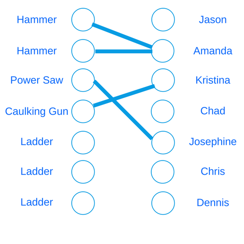
Now we want to find the “maximum matching” in this graph. That is, we want the largest set of edges such that no two edges share a node. The way to solve this problem using graph algorithms is to turn it into yet ANOTHER graph problem! We’ll add a node on the far left, called the “source” node. We’ll connect it to every “tool” node. Now we’ll add a node on the far right, called the “sink” node. It will receive an edge from every “person” node. All the edges in this graph have a distance of 1.

Again, most of the middle edges are missing here.

The size of the maximum matching in this case is equal to the “max flow” from the source node to the sink node. This is a somewhat advanced concept. But imagine there is water gushing out of the source node and that every edge is a “pipe” whose value (1) is the capacity. We want the largest amount of water that can go through to the sink at once.

Last week we saw built-in functions for shortest path and min spanning tree. FGL also has an out-of-the-box solution for max flow. So our main goal now is to take our objects and construct the above graph.

Preparing Our Solution

A couple weeks ago, we created a segment tree that was very specific to the problem. This time, we’ll show what it’s like to write a more generic algorithm. Throughout the rest of the article, you can imagine that a is a tool, and b is a person. We’ll write a general maxMatching function that will take a list of a’s, a list of b’s, AND a predicate function. This function will determine whether an a object and a b object should have an edge between them. We’ll use the containsTool function from above as our predicate. Then we'll call our general function.

findMaxMatchingBest :: [String] -> [(String, [String])] -> Int
findMaxMatchingBest tools personMap = findMaxMatching containsTool tools personMap

…(different module)

findMaxMatching :: (a -> b -> Bool) -> [a] -> [b] -> Int
findMaxMatching predicate as bs = ...

Building Our Graph

To build our graph, we’ll have to decide on our labels. Once again, we’ll only label our edges with integers. In fact, they’ll all have a “capacity” label of 1. But our nodes will be a little more complicated. We’ll want to associate the node with the object, and we have a heterogeneous (and polymorphic) set of items. We’ll make this NodeLabel type that could refer to any of the four types of nodes:

data NodeLabel a b = 
  LeftNode a |
  RightNode b |
  SourceNode |
  SinkNode

Next we’ll start building our graph by constructing the inner part. We’ll make the two sets of nodes as well as the edges connecting them. We’ll assign the left nodes to the indices from 1 up through the size of that list. And then the right nodes will take on the indices from one above the first list's size through the sum of the list sizes.

createInnerGraph 
  :: (a -> b -> Bool) 
  -> [a]
  -> [b]
  -> ([LNode (NodeLabel a b)], [LNode (NodeLabel a b)], [LEdge Int])
createInnerGraph predicate as bs = ...
  where
    sz_a = length as
    sz_b = length bs
    aNodes = zip [1..sz_a] (LeftNode <$> as)
    bNodes = zip [(sz_a + 1)..(sz_a + sz_b)] (RightNode <$> bs)

Next we’ll also make tuples matching the index to the item itself without its node label wrapper. This will allow us to call the predicate on these items. We’ll then get all the edges out by using a list comprehension. We'll pull each pairing and determining if the predicate holds. If it does, we’ll add the edge.

where
  ...
  indexedAs = zip [1..sz_a] as
  indexedBs = zip [(sz_a + 1)..(sz_a + sz_b)] bs
  nodesAreConnected (_, aItem) (_, bItem) = predicate aItem bItem
  edges = [(fst aN, fst bN, 1) | aN <- indexedAs, bN <- indexedBs, nodesAreConnected aN bN]

Now we’ve got all our pieces, so we combine them to complete the definition:

createInnerGraph predicate as bs = (aNodes, bNodes, edges)

Now we’ll construct the “total graph”. This will include the source and sink nodes. It will include the indices of these nodes in the return value so that we can use them in our algorithm:

totalGraph :: (a -> b -> Bool) -> [a] -> [b] 
  -> (Gr (NodeLabel a b) Int, Int, Int)

Now we’ll start our definition by getting all the pieces out of the inner graph as well as the size of each list. Then we’ll assign the index for the source and sink to be the numbers after these combined sizes. We’ll also make the nodes themselves and give them the proper labels.

totalGraph predicate as bs = ...
  where
    sz_a = length as
    sz_b = length bs
    (leftNodes, rightNodes, middleEdges) = createInnerGraph predicate as bs
    sourceIndex = sz_a + sz_b + 1
    sinkIndex = sz_a + sz_b + 2
    sourceNode = (sourceIndex, SourceNode)
    sinkNode = (sinkIndex, SinkNode)

Now to finish this definition, we’ll first create edges from the source out to the right nodes. Then we'll make edges from the left nodes to the sink. We’ll also use list comprehensions there. Then we’ll combine all our nodes and edges into two lists.

where
  ...
  sourceEdges = [(sourceIndex, lIndex, 1) | lIndex <- fst <$> leftNodes]
  sinkEdges = [(rIndex, sinkIndex, 1) | rIndex <- fst <$> rightNodes]
  allNodes = sourceNode : sinkNode : (leftNodes ++ rightNodes)
  allEdges = sourceEdges ++ middleEdges ++ sinkEdges

Finally, we’ll complete the definition by making our graph. As we noted, we'll also return the source and sink indices:

totalGraph predicate as bs = (mkGraph allNodes allEdges, sourceIndex, sinkIndex)
  where
    ...

The Grand Finale

OK one last step! We can now fill in our findMaxMatching function. We’ll first get the necessary components from building the graph. Then we’ll call the maxFlow function. This works out of the box, just like sp and msTree from the last article!

import Data.Graph.Inductive.Graph (LNode, LEdge, mkGraph)
import Data.Graph.Inductive.PatriciaTree (Gr)
import Data.Graph.Inductive.Query.MaxFlow (maxFlow)

findMaxMatching :: (a -> b -> Bool) -> [a] -> [b] -> Int
findMaxMatching predicate as bs = maxFlow graph source sink
  where
    (graph, source, sink) = totalGraph predicate as bs

And we’re done! This will always give us the correct answer and it runs very fast! Take a look at the code on Github if you want to experiment with it!

Conclusion

Whew algorithms are exhausting aren’t they? That was a ton of code we just wrote. Let’s do a quick review. So this time around we looked at an actual problem that was not an obvious graph problem. We even tried a couple different algorithmic approaches. They both had issues though. Ultimately, we found that a graph algorithm was the solution, and we were able to implement it with FGL.

If you want to use FGL (or most any awesome Haskell library), it would help a ton if you learned how to use Stack! This great tool wraps project organization and package management into one tool. Check out our FREE Stack mini-course and learn more!

If you’ve never programmed in Haskell at all, then what are you waiting for? It’s super fun! You should download our Getting Started Checklist for some tips and resources on starting out!

Stay tuned next week for more on the Monday Morning Haskell Blog!

Graphing it Out

In the last two articles we dealt with some algorithmic issues. We were only able to solve these by improving the data structures in our code. First we used Haskell's built in array type for fast indexing. Then when we needed a segment tree, and we decided to make it from scratch. But we can’t roll our own data structure for every problem we encounter. So it’s good to have some systems we can use for more of these advanced topics.

One of the most important categories of data structures we’ll need for algorithms is graphs. Graphs are quite powerful when it comes to representing complicated problems. They are very useful for expressing relationships between data points. In this article, we'll see two types of graph problems. We’ll learn all about a library called the Functional Graph Library (FGL) that is available on Hackage for us to use. We’ll then take a stab at constructing graphs using the library. Finally, we’ll see how simple it is to solve these algorithms using this library once we’ve made our graphs.

For a complete set of the code that we’ll use in this article, check out this Github repository. It’ll show you how you can use Stack to bring the Functional graph library into your code.

If you’ve never used Stack before, it’s an indispensible tool for creating programs in Haskell. You should try out our Stack mini-course and learn more about it.

Graphs 101

For those of you who aren’t familiar with graphs and graph algorithms, I’ll explain a few of the basics here. If you’re very familiar with these already, you can skip this section. A graph contains a series of objects and encodes various relationships between these objects. For each object in our set, we have a “node” in our graph. These are like data points. Then to represent every relationship, we create an “edge” between two different nodes. We often give some kind of value to this edge as a piece of information about the relationship. In this article, we’ll imagine our nodes as places on a map, with the edges representing legal routes between locations. The label of each edge is the distance.

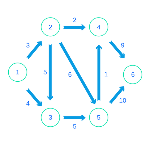
Edges can be both “directed” and “undirected”. Directed edges describe a 1-way relationship between the nodes. Undirected edges describe a 2-way relationship. Here's an example of a graph with directed edges:

Making Graphs with FGL

So whenever we’re making a graph with FGL, we’ll use a two-step process. First, we’ll create the “nodes” of our graph. Then we’ll encode the edges. Let’s suppose we’re reading an input stream. The stream will first give us the number of nodes and then edges in our graph. Then we’ll read a bunch of 3-tuples line-by-line. The first two numbers will refer to the "from" node and the "to" node. The third number will represent the distance. Here’s what this stream might look like for the graph pictured above:

6
9
1 2 3
1 3 4
2 3 5
2 4 2
2 5 6
3 5 5
4 6 9
5 4 1
5 6 10

We’ll read this input stream like so:

import Control.Monad (replicateM)
import System.IO (Handle, hGetLine)

data EdgeSpec = EdgeSpec
  { fromNode :: Int
  , toNode :: Int
  , distance :: Int
  }

readInputs :: Handle -> IO (Int, [EdgeSpec])
readInputs handle = do
  numNodes <- read <$> hGetLine handle
  numEdges <- (read <$> hGetLine handle)
  edges <- replicateM numEdges (readEdge handle)
  return (numNodes, edges)

readEdge :: Handle -> IO EdgeSpec
readEdge handle = do
  input <- hGetLine handle
  let [f_s, t_s, d_s] = words input
  return $ EdgeSpec (read f_s) (read t_s) (read d_s)

Our goal will be to encode this graph in the format of FGL. In this library, every node has an integer identifier. Nodes can either be “labeled” or “unlabeled”. This label, if it exists, is separate from the integer identifier. The function we’ll use requires our nodes to have labels, but we won’t need this extra information. So we’ll use a newtype to wrap the same integer identifier.

Once we know the number of nodes, it’s actually quite easy to create them all. We'll make labels from every number from 1 up through the length. Then we represent each node by the tuple of its index and label. Let’s start a function for creating our graph:

import Data.Graph.Inductive.Graph (mkGraph)
import Data.Graph.Inductive.PatriciaTree (Gr)

…

newtype NodeLabel = NodeLabel Int 
type Distance = Int

genGraph :: (Int, [EdgeSpec]) -> Gr NodeLabel Distance
genGraph (numNodes, edgeSpecs) = mkGraph nodes edges
  where
    nodes = (\i -> (i, NodeLabel i)) 
      <$> [1..numNodes]
    edges = ...

The graph we're making uses a "Patricia Tree" encoding under the hood. We won't go into details about that. We'll just call a simple mkGraph function exposed by the library. We'll make our return value the graph type Gr parameterized by our node label type and our edge label type. As we can see, we’ll use a type synonym Distance for integers to label our edges.

For now let’s get to the business of creating our edges. The format we specified with EdgeSpec works out that we don’t have to do much work. Just as the labeled node type is a synonym for a tuple, the labeled edge is a 3-tuple. It contains the indices of the “from” node, the “to” node, and then the distance label. In this case we’ll use directed edges. We do this for every edge spec, and then we’re done!

genGraph :: (Int, [EdgeSpec]) -> Gr NodeLabel Distance
genGraph (numNodes, edgeSpecs) = mkGraph nodes edges
  where
    nodes = (\i -> (i, NodeLabel i)) 
      <$> [1..numNodes]
    edges = (\es -> (fromNode es, toNode es, distance es))
      <$> edgeSpecs

Using Graph Algorithms

Now suppose we want to solve a particular graph problem. First we’ll tackle shortest path. If we remember from above, the shortest path from node 1 to node 6 on our graph actually just goes along the top, from 1 to 2 to 4 to 6.

How can we solve this from Haskell? We’ll first we’ll use our functions from above to read in the graph. Then we’ll imagine reading in two more numbers for the start and end nodes.

solveSP :: Handle -> IO ()
solveSP handle = do
  inputs <- readInputs handle
  start <- read <$> hGetLine handle
  end <- read <$> hGetLine handle
  let gr = genGraph inputs

Now with FGL we can simply make a couple library calls and we’ll get our results! We’ll use the Query.SP module, which exposes functions to find the shortest path and its length:

import Data.Graph.Inductive.Query.SP (sp, spLength)

solveSP :: Handle -> IO ()
solveSP handle = do
  inputs <- readInputs handle
  start <- read <$> hGetLine handle
  end <- read <$> hGetLine handle
  let gr = genGraph inputs
  print $ sp start end gr
  print $ spLength start end gr

We’ll get our output, which contains a representation of the path as well as the distance. Imagine “input.txt” contains our sample input above, except with two more lines for the start and end nodes “1” and “6”:

>> find-shortest-path < input.txt
[1,2,4,6]
14

We could change our file to instead go from 3 to 6, and then we’d get:

>> find-shortest-path < input2.txt
[3,5,4,6]
15

Cool!

Minimum Spanning Tree

Now let’s imagine a different problem. Suppose our nodes are internet hubs. We only want to make sure they’re all connected to each other somehow. We’re going to pick a subset of the edges that will create a “spanning tree”, connecting all our nodes. Of course, we want to do this in the cheapest way, by using the smallest total “distance” from the edges. This will be our “Minimum Spanning Tree”. First, let’s remove the directions on all the arrows. We can visualize this solution by looking at this picture, and we’ll see that we can connect our nodes at a total cost of 19.

The great news is that it’s not much more work to code this! First, we’ll adjust our graph construction a bit. To have an “undirected” graph in this scenario, we can make our arrows bi-directional like so:

genUndirectedGraph :: (Int, [EdgeSpec]) -> Gr NodeLabel Distance
genUndirectedGraph (numNodes, edgeSpecs) = mkGraph nodes edges
  where
    nodes = (\i -> (i, NodeLabel i)) 
      <$> [1..numNodes]
    edges = concatMap (\es -> 
      [(fromNode es, toNode es, distance es), (toNode es, fromNode es, distance es)])
      edgeSpecs

Besides this, all we have to do now is use the msTree function from the MST module! Then we'll get our result!

import Data.Graph.Inductive.Query.MST (msTree)

...

solveMST :: Handle -> IO ()
solveMST handle = do
  inputs <- readInputs handle
  let gr = genUndirectedGraph inputs
  print $ msTree gr

{- GHC Output
>> find-mst < “input1.txt”
[[(1,0)],[(2,3),(1,0)],[(4,2),(2,3),(1,0)],[(5,1),(4,2),(2,3),(1,0)],[(3,4),(1,0)],[(6,9),(4,2),(2,3),(1,0)]]
-}

This output is a little difficult to interpret, but it’s identical to the tree we saw above. Our output is a list of lists. Each sub-list contains a path from a node to our first node. A path list has a series of tuples, with each tuple corresponding to an edge. The first element of the tuple is the starting node, and the second is the distance.

So the first element, [(1,0)] refers to how node 1 connects to itself, by a single “edge” of distance 0 starting at 1. Then if we look at the last entry, we see node 6 connects to node 1 via a path through nodes 4 and 2, with total distance 9, 2, and 3.

Conclusion

Graph problems are ubiquitous in programming, but it can be a little tricky to get them right. It can be a definite pain to write your own graph data structure from scratch. It can be even harder to write out a full algorithm, even a well known one like Dijkstra's Algorithm. In Haskell, you can use the functional graph library to streamline this process. It has a built in format for representing the graph itself. It can be a little tedious to build up this structure. But once you have it, it’s actually very easy to solve many different common problems.

Next week, we’ll do a bit more work with FGL. We’ll explore a problem that isn’t quite as cut-and-dried as the ones we looked at here. First we'll take a more abstract problem and determine what graph we want to make for it. Then we'll solve that graph problem using FGL. So check back next week on the Monday Morning Haskell blog!.

The easiest way to bring FGL into your Haskell code is to use the Stack tool. If you’re unfamiliar with this, you should take our free Stack mini-course. You’ll learn the important step of how to bring dependencies into your code. You’ll also see the different components in a Stack program and the commands you can run to manipulate them.

If you’ve never programmed in Haskell before, you should try it! Download our Getting Started Checklist. It’ll point you towards some valuable resources in your early Haskell education.

Defeating Evil with Data Structures!

In last week’s article, we used benchmarks to determine how well our code performs on certain inputs. First we used the Criterion library to get some measurements for our code. Then we were able to look at those measurements in some spiffy output. We also profiled our code to try to determine what part of our code was slowing us down.

The profiling output highlighted two functions that were taking an awful lot of time. When we analyzed them, we found they were very inefficient. In this article, we’ll resolve those problems and improve our code in a couple different ways. First, we’ll use an array rather than a list to make our value accesses faster. Then, we’ll add a cool data structure called a segment tree. This will help us to quickly get the smallest height value over a particular interval.

The code examples in this article series make good use of the Stack tool. If you’ve never used Stack before, you should check out our new FREE Stack mini-course. It’ll walk you through the basics of organizing your code, getting dependencies, and running commands.

What Went Wrong?

So first let’s take some time to remind ourselves why these functions were slowing us down a lot. Both our minimum height function and our value at index function ran in O(n) time. This means each of them could scan the entire list in the worst case. Next we observed that both of these functions will get called O(n) times. Thus our total algorithm will be O(n^2) time. The time benchmarks we took backed up this theory.

The data structures we mentioned above will help us get the values we need without doing a full scan. We'll start by substituting in an array for our list, since that is a great deal easier.

Arrays

Linked lists are very common when we’re solving functional programming problems. They have some nice properties, and work very well with recursion. However, they do not allow fast access by index. For these situations, we need to use arrays. Arrays aren't as common in Haskell as other languages, and there are a few differences.

First, Haskell arrays have two type parameters. When you make an array in Java, you say whether it’s an int array (int[]) or a string array (String[]), or whatever other type. So this is only a single parameter. Whenever we want to index into the array, we always use integers.

In Haskell, we get to choose both the type that the array stores AND the type that indexes the array. Now, the indexing type has to belong to the index (Ix) typeclass. And in this case we’ll be using Int anyways. But it’s cool to know that you have more flexibility. For instance, consider representing a matrix. In Java, we have to use an “array of arrays”. This involves a lot of awkward syntax. In Haskell, we can instead use a single array indexed by tuples of integers! We could also do something like index from 1 instead of 0 if we wanted.

So for our problem, we’ll use Array Int Int for our inner fence values instead of a normal list. We'll only need to make a few code changes though! First, we'll import a couple modules and change our type to use the array:

import Data.Array
import Data.Ix (range)

...

newtype FenceValues = FenceValues { unFenceValues :: Array Int Int }

Next, instead of using (!!) to access by index, we’ll use the specialized array index (!) operator to access them.

valueAtIndex :: FenceValues -> FenceIndex -> Int
valueAtIndex values index = (unFenceValues values) ! (unFenceIndex index)

Finally, let's improve our minimumHeight function. We’ll now use the range function on our array instead of resorting to drop and take. Note we now use right - 1 since we want to exclude the right endpoint of the interval.

where
    valsInInterval :: [(FenceIndex, Int)]
    valsInInterval = zip 
      (FenceIndex <$> intervalRange) 
      (map ((unFenceValues values) !) intervalRange)
      where
        intervalRange = range (left, right - 1)

We’ll also have to change our benchmarking code to produce arrays instead of lists:

import Data.Array(listArray)

…

randomList :: Int -> IO FenceValues
randomList n = FenceValues . mkListArray <$> 
  (sequence $ replicate n (randomRIO (1, 10000 :: Int)))
  where
    mkListArray vals = listArray (0, (length vals) - 1) vals

Both our library and our benchmark now need to use array in their build-depends section of the Cabal file. We need to make sure we add this! Once we have, we can benchmark our code again, and we’ll find it’s already sped up quite a bit!

>> stack bench --profile
Running 1 benchmarks...
Benchmark fences-benchmarks: RUNNING...
benchmarking fences tests/Size 1 Test
time                 49.33 ns   (48.98 ns .. 49.71 ns)
                     1.000 R²   (0.999 R² .. 1.000 R²)
mean                 49.46 ns   (49.16 ns .. 49.86 ns)
std dev              1.105 ns   (861.0 ps .. 1.638 ns)
variance introduced by outliers: 33% (moderately inflated)

benchmarking fences tests/Size 10 Test
time                 4.541 μs   (4.484 μs .. 4.594 μs)
                     0.999 R²   (0.998 R² .. 1.000 R²)
mean                 4.496 μs   (4.456 μs .. 4.531 μs)
std dev              132.0 ns   (109.6 ns .. 164.3 ns)
variance introduced by outliers: 36% (moderately inflated)

benchmarking fences tests/Size 100 Test
time                 79.81 μs   (79.21 μs .. 80.45 μs)
                     0.999 R²   (0.999 R² .. 1.000 R²)
mean                 79.51 μs   (78.93 μs .. 80.39 μs)
std dev              2.396 μs   (1.853 μs .. 3.449 μs)
variance introduced by outliers: 29% (moderately inflated)

benchmarking fences tests/Size 1000 Test
time                 1.187 ms   (1.158 ms .. 1.224 ms)
                     0.995 R²   (0.992 R² .. 0.998 R²)
mean                 1.170 ms   (1.155 ms .. 1.191 ms)
std dev              56.61 μs   (48.02 μs .. 70.28 μs)
variance introduced by outliers: 37% (moderately inflated)

benchmarking fences tests/Size 10000 Test
time                 15.03 ms   (14.71 ms .. 15.32 ms)
                     0.997 R²   (0.994 R² .. 0.999 R²)
mean                 15.71 ms   (15.44 ms .. 16.03 ms)
std dev              729.7 μs   (569.3 μs .. 965.4 μs)
variance introduced by outliers: 16% (moderately inflated)

benchmarking fences tests/Size 100000 Test
time                 191.4 ms   (189.2 ms .. 193.9 ms)
                     1.000 R²   (1.000 R² .. 1.000 R²)
mean                 189.3 ms   (188.2 ms .. 190.5 ms)
std dev              1.471 ms   (828.0 μs .. 1.931 ms)
variance introduced by outliers: 14% (moderately inflated)

Benchmark fences-benchmarks: FINISH

Here’s what the multiplicative factors are:

Size 1: 49.33 ns
Size 10: 4.451 μs (increased ~90x)
Size 100: 79.81 μs (increased ~18x)
Size 1000: 1.187 ms (increased ~15x)
Size 10000: 15.03 ms (increased ~13x)
Size 100000: 191.4 ms (increased ~13x)

For the later cases, increasing size by a factor 10 seems to only increase the time by a factor of 13-15. We could be forgiven for thinking we have achieved O(n log n) time already!

Better Test Cases

But something still doesn't sit right. We have to remember that the theory doesn’t quite justify our excitement here. In fact our old code was SO BAD that the NORMAL case was O(n^2). Now it seems like we may have gotten O(n log n) for the average case. But we want to prepare for the worst case if we can. Imagine our code is being used by our evil adversary:

He’ll find the worst possible case! In this situation, our code will not be so performant when the lists of input heights is sorted!

main :: IO ()
main = do
  [l1, l2, l3, l4, l5, l6] <- mapM 
    randomList [1, 10, 100, 1000, 10000, 100000]
  let l7 = sortedList
  defaultMain
    [ bgroup "fences tests" 
        ...
       , bench "Size 100000 Test" $ whnf largestRectangle l6
      , bench "Size 100000 Test (sorted)" $ whnf largestRectangle l7
      ]
    ]

...

sortedList :: FenceValues
sortedList = FenceValues $ listArray (0, 99999) [1..100000]

We’ll once again find that this last case takes a loooong time, and we’ll see a big spike in run time.

>> stack bench --profile
Running 1 benchmarks...
Benchmark fences-benchmarks: RUNNING...

…

benchmarking fences tests/Size 100000 Test (sorted)
time                 378.1 s    (355.0 s .. 388.3 s)
                     1.000 R²   (0.999 R² .. 1.000 R²)
mean                 384.5 s    (379.3 s .. 387.2 s)
std dev              4.532 s    (0.0 s .. 4.670 s)
variance introduced by outliers: 19% (moderately inflated)

Benchmark fences-benchmarks: FINISH

It averages more than 6 minutes per case! But this time, we’ll see the profiling output has changed. It only calls out various portions of minimumHeightIndexValue! We no longer spend a lot of time in valueAtIndex.

COST CENTRE                                          %time %alloc

minimumHeightIndexValue.valsInInterval               65.0   67.7
minimumHeightIndexValue                              22.4    0.0
minimumHeightIndexValue.valsInInterval.intervalRange 12.4   32.2

So now we have to solve this new problem by improving our calculation of the minimum.

Segment Trees

Our current approach still requires us to look at every element in our interval. Even though some of our intervals will be small, there will be a lot of these smaller calls, so the total time is still O(n^2). We need a way to find the smallest item and value on a given interval without resorting to a linear scan.

One idea would be to develop an exhaustive list of all the answers to this question right at the start. We could make a mapping from all possible intervals to the smallest index and value in the interval. But this won’t help us in the end. There are still n^2 possible intervals. So creating this data structure will still mean that our code takes O(n^2) time.

But we’re on the right track with the idea of doing some of the work before hand. We'll have to use a data structure that’s not an exhaustive listing though. Enter segment trees.

A segment tree has the same structure as a binary search tree. Instead of storing a single value though, each node corresponds to an interval. Each node will store its interval, the smallest value over that interval, and the index of that value.

The top node on the tree will refer to the interval of the whole array. It'll store the pair for the smallest value and index overall. Then it will have two children nodes. The left one will have the minimum pair over the first half of the tree, and the right one will have the second half. The next layer will break it up into quarters, and so on.

As an example, let's consider how we would determine the minimum pair starting from the first quarter point and ending at the third quarter point. We’ll do this using recursion. First, we'll ask the left subtree for the minimum pair on the interval from the quarter point to the half point. Then we’ll query the right tree for the smallest pair from the half point to the three-quarters point. Then we can take the smallest of those and return it. I won’t go into all the theory here, but it turns out that even in the worst case this operation takes O(log n) time.

Designing Our Segment Tree

There is a library called Data.SegmentTree on hackage. But I thought it would be interesting to implement this data structure from scratch. We'll compose our tree from SegmentTreeNodes. Each node is either empty, or it contains six fields. The first two refer to the interval the node spans. The next will be the minimum value and the index of that value over the interval. And then we’ll have fields for each of the children nodes of this node:

data SegmentTreeNode = ValueNode
  { fromIndex :: FenceIndex
  , toIndex :: FenceIndex
  , value :: Int
  , minIndex :: FenceIndex
  , leftChild :: SegmentTreeNode
  , rightChild :: SegmentTreeNode
  }
  | EmptyNode

We could make this Segment Tree type a lot more generic so that it isn’t restricted to our fence problem. I would encourage you to take this code and try that as an exercise!

Building the Segment Tree

Now we’ll add our preprocessing step where we’ll actually build the tree itself. This will use the same interval/tail pattern we saw before. In the base case, the interval’s span is only 1, so we make a node containing that value with empty sub-children. We’ll also add a catchall that returns an EmptyNode:

buildSegmentTree :: Array Int Int -> SegmentTreeNode
buildSegmentTree ints = buildSegmentTreeTail 
  ints 
  (FenceInterval ((FenceIndex 0), (FenceIndex (length (elems ints)))))

buildSegmentTreeTail :: Array Int Int -> FenceInterval -> SegmentTreeNode
buildSegmentTreeTail array
  (FenceInterval (wrappedFromIndex@(FenceIndex fromIndex), wrappedToIndex@(FenceIndex toIndex)))
  | fromIndex + 1 == toIndex = ValueNode 
      { fromIndex = wrappedFromIndex
      , toIndex = wrappedToIndex
      , value = array ! fromIndex
      , minIndex = wrappedFromIndex
      , leftChild = EmptyNode
      , rightChild = EmptyNode
      }
  | … missing case
  | otherwise = EmptyNode

Now our middle case will be the standard case. First we’ll divide our interval in half and make two recursive calls.

where 
  average = (fromIndex + toIndex) `quot` 2
  -- Recursive Calls
  leftChild = buildSegmentTreeTail 
    array (FenceInterval (wrappedFromIndex, (FenceIndex average)))
  rightChild = buildSegmentTreeTail 
    array (FenceInterval ((FenceIndex average), wrappedToIndex))

Next we’ll write a function that’ll extract the minimum value and index, but handle the empty node case:

-- Get minimum val and index, but account for empty case.
valFromNode :: SegmentTreeNode -> (Int, FenceIndex)
valFromNode EmptyNode = (maxBound :: Int, FenceIndex (-1))
valFromNode n@ValueNode{} = (value n, minIndex n)

Now we’ll compare the three cases for the this minimum. It’ll likely be the values from the left or the right. Otherwise it’s the current value.

leftCase = valFromNode leftChild
rightCase = valFromNode rightChild
currentCase = (array ! fromIndex, wrappedFromIndex)
(newValue, newIndex) = min (min leftCase rightCase) currentCase

Finally we’ll complete our definition by filling in the missing variables in the middle/normal case. Here’s the full function:

buildSegmentTreeTail :: Array Int Int -> FenceInterval -> SegmentTreeNode
buildSegmentTreeTail array
  (FenceInterval (wrappedFromIndex@(FenceIndex fromIndex), wrappedToIndex@(FenceIndex toIndex)))
  | fromIndex + 1 == toIndex = ValueNode 
      { fromIndex = wrappedFromIndex
      , toIndex = wrappedToIndex
      , value = array ! fromIndex
      , minIndex = wrappedFromIndex
      , leftChild = EmptyNode
      , rightChild = EmptyNode
      }
  | fromIndex < toIndex = ValueNode 
    { fromIndex = wrappedFromIndex
    , toIndex = wrappedToIndex
    , value = newValue
    , minIndex = newIndex
    , leftChild = leftChild
    , rightChild = rightChild
    }
  | otherwise = EmptyNode
    where 
      average = (fromIndex + toIndex) `quot` 2
      -- Recursive Calls
      leftChild = buildSegmentTreeTail 
        array (FenceInterval (wrappedFromIndex, (FenceIndex average)))
      rightChild = buildSegmentTreeTail 
        array (FenceInterval ((FenceIndex average), wrappedToIndex))

      -- Get minimum val and index, but account for empty case.
      valFromNode :: SegmentTreeNode -> (Int, FenceIndex)
      valFromNode EmptyNode = (maxBound :: Int, FenceIndex (-1))
      valFromNode n@ValueNode{} = (value n, minIndex n)

      leftCase = valFromNode leftChild
      rightCase = valFromNode rightChild
      currentCase = (array ! fromIndex, wrappedFromIndex)
      (newValue, newIndex) = min (min leftCase rightCase) currentCase

Finding the Minimum

Now let’s write the critical function of finding the minimum over the given interval. We’ll add our tree as another parameter. Then we’ll handle the EmptyNode case and then unwrap our values for the full case:

minimumHeightIndexValue :: FenceValues -> SegmentTreeNode -> FenceInterval -> (FenceIndex, Int)
minimumHeightIndexValue values tree 
  originalInterval@(FenceInterval (FenceIndex left, FenceIndex right)) =
  case tree of
    EmptyNode -> (maxBound :: Int, -1)
    ValueNode
      { fromIndex = FenceIndex nFromIndex
      , toIndex = FenceIndex nToIndex
      , value = nValue
      , minIndex = nMinIndex
      , leftChild = nLeftChild
      , rightChild = nRightChild} ->

Next we’ll handle the base case that we are at exactly the correct node:

| left == nFromIndex && right == nToIndex = (nValue, nMinIndex)

Next we’ll observe two cases that will need only one recursive call. If the right index is below the midway point, we recursively call to the left sub-child. And if the left index is above the midway point, we’ll call on the right side (we’ll calculate the average later).

| otherwise = if right < average 
  then minimumHeightIndexValue values nLeftChild originalInterval
  else if left >= average
    then minimumHeightIndexValue values nRightChild originalInterval

Finally we have a tricky part. If the interval does cross the halfway mark, we’ll have to divide it into two sub-intervals. Then we’ll make two recursive calls, and get their solutions. Finally, we’ll compare the two solutions and take the smaller one.

else minTuple leftResult rightResult
  where
    average = (nFromIndex + nToIndex) `quot` 2
    leftResult = minimumHeightIndexValue values nLeftChild
      (FenceInterval (FenceIndex left, FenceIndex average))
    rightResult = minimumHeightIndexValue values nRightChild
      (FenceInterval (FenceIndex average, FenceIndex right))
    minTuple :: (FenceIndex, Int) -> (FenceIndex, Int) -> (FenceIndex, Int)
    minTuple old@(_, heightOld) new@(_, heightNew) =
      if heightNew < heightOld then new else old

Here’s the full function for clarity:

minimumHeightIndexValue :: FenceValues -> SegmentTreeNode -> FenceInterval -> (FenceIndex, Int)
minimumHeightIndexValue values tree 
  originalInterval@(FenceInterval (FenceIndex left, FenceIndex right)) =
  case tree of
    EmptyNode -> (maxBound :: Int, -1)
    ValueNode
      { fromIndex = FenceIndex nFromIndex
      , toIndex = FenceIndex nToIndex
      , value = nValue
      , minIndex = nMinIndex
      , leftChild = nLeftChild
      , rightChild = nRightChild} ->
        | left == nFromIndex && right == nToIndex = (nValue, nMinIndex)
        | otherwise = if right < average 
          then minimumHeightIndexValue values nLeftChild originalInterval
          else if left >= average
            then minimumHeightIndexValue values nRightChild originalInterval
            else minTuple leftResult rightResult
          where
            average = (nFromIndex + nToIndex) `quot` 2
            leftResult = minimumHeightIndexValue values nLeftChild
              (FenceInterval (FenceIndex left, FenceIndex average))
            rightResult = minimumHeightIndexValue values nRightChild
              (FenceInterval (FenceIndex average, FenceIndex right))
          minTuple :: (FenceIndex, Int) -> (FenceIndex, Int) -> (FenceIndex, Int)
          minTuple old@(_, heightOld) new@(_, heightNew) =
            if heightNew < heightOld then new else old

Touching Up the Rest

Once we’ve accomplished this, the rest is pretty straightforward. First, we’ll build our segment tree at the beginning and pass that as a parameter to our function. Then we’ll plug in our new minimum function in place of the old one. We’ll make sure to add the tree to each recursive call as well.

largestRectangle :: FenceValues -> FenceSolution
largestRectangle values = largestRectangleAtIndices values 
  (buildSegmentTree (unFenceValues values)
  (FenceInterval (FenceIndex 0, FenceIndex (length (unFenceValues values))))

…
-- Notice the extra parameter
largestRectangleAtIndices :: FenceValues -> SegmentTreeNode -> FenceInterval -> FenceSolution
largestRectangleAtIndices
  values
  tree
…
      where
      …
      -- And down here add it to each call
      (minIndex, minValue) = minimumHeightIndexValue values tree interval
      leftCase = largestRectangleAtIndices values tree (FenceInterval (leftIndex, minIndex))
      rightCase = if minIndex + 1 == rightIndex
        then FenceSolution (maxBound :: Int)
        else largestRectangleAtIndices values tree (FenceInterval (minIndex + 1, rightIndex))

And now we can run our benchmarks again. This time, we’ll see that our code runs a great deal faster on both large cases! Success!

benchmarking fences tests/Size 100000 Test
time                 179.1 ms   (173.5 ms .. 185.9 ms)
                     0.999 R²   (0.998 R² .. 1.000 R²)
mean                 184.1 ms   (182.7 ms .. 186.1 ms)
std dev              2.218 ms   (1.197 ms .. 3.342 ms)
variance introduced by outliers: 14% (moderately inflated)

benchmarking fences tests/Size 100000 Test (sorted)
time                 238.4 ms   (227.2 ms .. 265.1 ms)
                     0.998 R²   (0.989 R² .. 1.000 R²)
mean                 243.5 ms   (237.0 ms .. 251.8 ms)
std dev              8.691 ms   (2.681 ms .. 11.83 ms)
variance introduced by outliers: 16% (moderately inflated)

Conclusion

So in these past two articles we’ve learned a whole lot. We first covered how to create benchmarks for our code using Cabal/Stack. When we ran those benchmarks, we found results took longer than we would like. We then used profiling to determine what the problematic functions were. Then we dove head-first into some data structures knowledge. We saw first hand how changing the underlying data structures of our program could improve our performance. We also learned about arrays, which are somewhat overlooked in Haskell. Then we built a segment tree from scratch and used its API to enable our program’s improvements.

This problem involved many different uses of recursion. If you want to become a better functional programmer, you’d better learn recursion. If you want a better grasp of this fundamental concept, you should check out our FREE Recursion Workbook. It has two chapters of useful information as well as 10 practice problems!

If you’ve never written Haskell before but are intrigued by the possibilities you saw in this article, you should try it out! Download our Getting Started Checklist! It’ll walk you through installing the language. It'll also point you to some cool resources for starting your Haskell education.

Finally, be sure to check out our Stack mini-course. Once you’ve mastered the Stack tool, you’ll be well on your way to making Haskell projects like a Pro!

How well does it work? Profiling in Haskell

I’ve said it before, but I’ll say it again. As much as we’d like to think it’s the case, our Haskell code doesn’t work just because it compiles. This is why we have test suites. But even if it passes our test suites this doesn’t mean it works as well as it could either. Sometimes we’ll realize that the code we wrote isn’t quite performant enough, so we’ll have to make improvements.

But improving our code can sometimes feel like taking shots in the dark. You'll spend a great deal of time tweaking a certain piece. Then you'll find you haven’t actually made much of a dent in the total run time of the application. Certain operations generally take longer, like database calls, network operations, and IO. So you can often have a decent idea of where to start. But it always helps to be sure. This is where benchmarking and profiling come in. We’re going to take a specific problem and learn how we can use some Haskell tools to zero in on the problem point.

As a note, the tools we’ll use require you to be organizing your code using Stack or Cabal. If you’ve never used either of these before, you should check out our Stack Mini Course! It'll teach you the basics of creating a project with Stack. You'll also learn the primary commands to use with Stack. It’s brand new and best of all FREE! Check it out! It’s our first course of any kind, so we’re looking for feedback!

The Problem

Our overarching problem for this article will be the “largest rectangle” problem. You can actually try to solve this problem yourself on Hackerrank under the name “John and Fences”. Imagine we have a series of vertical bars with varying heights placed next to each other. We want to find the area of the largest rectangle that we can draw over these bars that doesn’t include any empty space. Here’s a visualization of one such problem and solution:

In this example, we have posts with heights [2,5,7,4,1,8]. The largest rectangle we can form has an area of 12, as we see with the highlighted squares.

This problem is pretty neat and clean to solve with Haskell, as it lends itself to a recursive solution. First let’s define a couple newtypes to illustrate our concepts for this problem. We’ll use a compiler extension to derive the Num typeclass on our index type, as this will be useful later.

{-# LANGUAGE GeneralizedNewtypeDeriving #-}
...
newtype FenceValues = FenceValues { unFenceValues :: [Int] }
newtype FenceIndex = FenceIndex { unFenceIndex :: Int }
  deriving (Eq, Num, Ord)
-- Left Index is inclusive, right index is non-inclusive 
newtype FenceInterval = FenceInterval { unFenceInterval :: (FenceIndex, FenceIndex) }
newtype FenceSolution = FenceSolution { unFenceSolution :: Int }
  deriving (Eq, Show, Ord)

Next, we’ll define our primary function. It will take our FenceValues, a list of integers, and return our solution.

largestRectangle :: FenceValues -> FenceSolution
largestRectangle values = ...

It in turn will call our recursive helper function. This function will calculate the largest rectangle over a specific interval. We can solve it recursively by using smaller and smaller intervals. We’ll start by calling it on the interval of the whole list.

largestRectangle :: FenceValues -> FenceSolution
largestRectangle values = largestRectangleAtIndices values
  (FenceInterval (FenceIndex 0, FenceIndex (length (unFenceValues values))))

largestRectangleAtIndices :: FenceValues -> FenceInterval -> FenceSolution
largestRectangleAtIndices = ...

Now, to break this into recursive cases, we need some more information first. What we need is the index i of the minimum height in this interval. One option is that we could make a rectangle spanning the whole interval with this height.

Any other "largest rectangle" won't use this particular index. So we can then divide our problem into two more cases. In the first, we'll find the largest rectangle on the interval to the left. In the second, we'll look to the right.

As your might realize, these two cases simply involve making recursive calls! Then we can easily compare their results. The only thing we need to add is a base case. Here are all these cases represented in code:

largestRectangleAtIndices :: FenceValues -> FenceInterval -> FenceSolution
largestRectangleAtIndices
  values
  interval@(FenceInterval (leftIndex, rightIndex)) = 
    -- Base Case: Checks if left + 1 >= right
    if isBaseInterval interval
      then FenceSolution (valueAtIndex values leftIndex)
      -- Compare three cases
      else max (max middleCase leftCase) rightCase
      where
      -- Find the minimum height and its index
      (minIndex, minValue) = minimumHeightIndexValue values interval
      -- Case 1: Use the minimum index
      middleCase = FenceSolution $ (intervalSize interval) * minValue
      -- Recursive call #1
      leftCase = largestRectangleAtIndices values (FenceInterval (leftIndex, minIndex))
      -- Guard against case where there is no "right" interval
      rightCase = if minIndex + 1 == rightIndex
        then FenceSolution (maxBound :: Int) -- Supply a "fake" solution that we'll ignore
        -- Recursive call #2
        else largestRectangleAtIndices values (FenceInterval (minIndex + 1, rightIndex))

And just like that, we’re actually almost finished. The only sticking point here is a few helper functions. Three of these are simple:

valueAtIndex :: FenceValues -> FenceIndex -> Int
valueAtIndex values index = (unFenceValues values) !! (unFenceIndex index)

isBaseInterval :: FenceInterval -> Bool
isBaseInterval (FenceInterval (FenceIndex left, FenceIndex right)) = left + 1 >= right

intervalSize :: FenceInterval -> Int
intervalSize (FenceInterval (FenceIndex left, FenceIndex right)) = right - left

Now we have to determine the minimum on this interval. Let’s do this in the most naive way, by scanning the whole interval with a fold.

minimumHeightIndexValue :: FenceValues -> FenceInterval -> (FenceIndex, Int)
minimumHeightIndexValue values (FenceInterval (FenceIndex left, FenceIndex right)) =
  foldl minTuple (FenceIndex (-1), maxBound :: Int) valsInInterval
  where
    valsInInterval :: [(FenceIndex, Int)]
    valsInInterval = drop left (take right (zip (FenceIndex <$> [0..]) (unFenceValues values)))
    minTuple :: (FenceIndex, Int) -> (FenceIndex, Int) -> (FenceIndex, Int)
    minTuple old@(_, heightOld) new@(_, heightNew) =
      if heightNew < heightOld then new else old

And now we’re done!

Benchmarking our Code

Now, this is a neat little algorithmic solution, but we want to know if our code is efficient. We need to know if it will scale to larger input values. We can find the answer to this question by writing benchmarks. Benchmarks are a feature we can use in conjunction with Cabal and Stack. They work a lot like test suites. But instead of proving the correctness of our code, they’ll show us how fast our code runs under various circumstances. We’ll use the Criterion library to do this. We’ll start by adding a section in our .cabal file for this benchmark:

benchmark fences-benchmarks
  type:                exitcode-stdio-1.0
  hs-source-dirs:      benchmark
  main-is:             fences-benchmark.hs
  build-depends:       base
                     , FencesExample
                     , criterion
                     , random
  default-language:    Haskell2010

Now we’ll make our file fences-benchmark.hs, make it a Main module and add a main function. We’ll generate 6 lists, increasing in size by a factor of 10 each time. Then we’ll create a benchmark group and call the bench function on each situation.

module Main where

import Criterion
import Criterion.Main (defaultMain)
import System.Random

import Lib

main :: IO ()
main = do
  [l1, l2, l3, l4, l5, l6] <- mapM 
    randomList [1, 10, 100, 1000, 10000, 100000]
  defaultMain
    [ bgroup "fences tests" 
      [ bench "Size 1 Test" $ whnf largestRectangle l1
      , bench "Size 10 Test" $ whnf largestRectangle l2
      , bench "Size 100 Test" $ whnf largestRectangle l3
      , bench "Size 1000 Test" $ whnf largestRectangle l4
      , bench "Size 10000 Test" $ whnf largestRectangle l5
      , bench "Size 100000 Test" $ whnf largestRectangle l6
      ]
    ]

-- Generate a list of a particular size
randomList :: Int -> IO FenceValues
randomList n = FenceValues <$> (sequence $ replicate n (randomRIO (1, 10000 :: Int)))

We’d normally run these benchmarks with stack bench (or cabal bench if you’re not using Stack). But we can also compile our code with the --profile flag. This will automatically create a profiling report with more information about our code. Note using profiling requires re-compiling ALL the dependencies to use profiling as well. So you don't want to switch back and forth a lot.

>> stack bench --profile
Benchmark fences-benchmarks: RUNNING...
benchmarking fences tests/Size 1 Test
time                 47.79 ns   (47.48 ns .. 48.10 ns)
                     1.000 R²   (0.999 R² .. 1.000 R²)
mean                 47.78 ns   (47.48 ns .. 48.24 ns)
std dev              1.163 ns   (817.2 ps .. 1.841 ns)
variance introduced by outliers: 37% (moderately inflated)

benchmarking fences tests/Size 10 Test
time                 3.324 μs   (3.297 μs .. 3.356 μs)
                     0.999 R²   (0.999 R² .. 1.000 R²)
mean                 3.340 μs   (3.312 μs .. 3.368 μs)
std dev              98.52 ns   (79.65 ns .. 127.2 ns)
variance introduced by outliers: 38% (moderately inflated)

benchmarking fences tests/Size 100 Test
time                 107.3 μs   (106.3 μs .. 108.2 μs)
                     0.999 R²   (0.999 R² .. 0.999 R²)
mean                 107.2 μs   (106.3 μs .. 108.4 μs)
std dev              3.379 μs   (2.692 μs .. 4.667 μs)
variance introduced by outliers: 30% (moderately inflated)

benchmarking fences tests/Size 1000 Test
time                 8.724 ms   (8.596 ms .. 8.865 ms)
                     0.998 R²   (0.997 R² .. 0.999 R²)
mean                 8.638 ms   (8.560 ms .. 8.723 ms)
std dev              228.8 μs   (193.6 μs .. 272.8 μs)

benchmarking fences tests/Size 10000 Test
time                 909.2 ms   (899.3 ms .. 914.1 ms)
                     1.000 R²   (1.000 R² .. 1.000 R²)
mean                 915.1 ms   (914.6 ms .. 915.8 ms)
std dev              620.1 μs   (136.0 as .. 664.8 μs)
variance introduced by outliers: 19% (moderately inflated)

benchmarking fences tests/Size 100000 Test
time                 103.9 s    (91.11 s .. 117.3 s)
                     0.997 R²   (0.997 R² .. 1.000 R²)
mean                 107.3 s    (103.7 s .. 109.4 s)
std dev              3.258 s    (0.0 s .. 3.702 s)
variance introduced by outliers: 19% (moderately inflated)

Benchmark fences-benchmarks: FINISH

So when we run this, we’ll find something...troubling. It takes a looong time to run the final benchmark on size 100000. On average, this case takes over 100 seconds...more than a minute and a half! We can further take note of how the average run time increases based on the size of the case. Let’s pare down the data a little bit:

Size 1: 47.78 ns
Size 10: 3.340 μs (increased ~70x)
Size 100: 107.2 μs (increased ~32x)
Size 1000: 8.638 ms (increased ~81x)
Size 10000: 915.1 ms (increased ~106x)
Size 100000: 107.3 s (increased ~117x)

Each time we increase the size of the problem by a factor of 10, the time spent increased by a factor closer to 100! This suggests our run time is O(n^2) (check out this guide if you are unfamiliar with Big-O notation). We’d like to do better.

Determining the Problem

So we want to figure out why our code isn’t performing very well. Luckily, we already profiled our benchmark!. This outputs a specific file that we can look at, called fences-benchmark.prof. It has some very interesting results:

COST CENTRE                            MODULE SRC                 %time %alloc
minimumHeightIndexValue.valsInInterval Lib    src/Lib.hs:45:5-95   69.8   99.7
valueAtIndex                           Lib    src/Lib.hs:51:1-74   29.3    0.0

We see that we have two big culprits taking a lot of time. First, there is our function that determines the minimum between a specific interval. The report is even more specific, calling out the specific offending part of the function. We spend a lot of time getting the different values for a specific interval. In second place, we have valueAtIndex. This means we also spend a lot of time getting values out of our list.

First let’s be glad we’ve factored our code well. If we had written our entire solution in one big function, we wouldn’t have any leads here. This makes it much easier for us to analyze the problem. When examining the code, we see why both of these functions could produce O(n^2) behavior.

Due to the number of recursive calls we make, we’ll call each of these functions O(n) times. Then when we call valueAtIndex, we use the (!!) operator on our linked list. This takes O(n) time. Scanning the whole interval for the minimum height has the same effect. In the worst case, we have to look at every element in the list! I’m hand waving a bit here, but that is the basic result. When we call these O(n) pieces O(n) times, we get O(n^2) time total.

Cliff Hanger Ending

We can actually solve this problem in O(n log n) time, a dramatic improvement over the current O(n^2). But we’ll have to improve our data structures to accomplish this. First, we’ll store our values so that we can go from the index to the element in sub-linear time. This is easy. Second, we have to determine the index containing the minimum element within an arbitrary interval. This is a bit trickier to do in sub-linear time. We'll need a more advanced data structure.

To find out how we solve these problems, you’ll have to wait for part 2 of this series! Come back next week to the Monday Morning Haskell blog!

As a reminder, we’ve just published a FREE mini-course on Stack. It’ll teach you the basics of laying out a project and running commands on it using the Stack tool. You should enroll in the Monday Morning Haskell Academy to sign up! This is our first course of any kind, so we would love to get some feedback! Once you know about Stack, it'll be a lot easier to try this problem out for yourself!

In addition to Stack, recursion also featured pretty heavily in our solution here. If you’ve done any amount of functional programming you’ve seen recursion in action. But if you want to solidify your knowledge, you should download our FREE Recursion Workbook! It has two chapters worth of content on recursion and it has 10 practice problems you can work through!

Never programmed in Haskell? No problem! You can download our Getting Started Checklist and it’ll help you get Haskell installed. It’ll also point you in the direction of some great learning resources as well. Take a look!

Taking a Close look at Lenses

So when we first learned about creating our own data types, we went over the idea of record syntax. The idea of record syntax is pretty simple. We want to create objects with named fields. This allows us to avoid the tedium of pattern matching on objects all the time to get any kind of data out of them. Record syntax allows us to create functions that pull an individual field out of an object. Besides retrieving fields from an object, we can also create a modified object. We specify only the records we want to change.

data Task = Task
  { taskName :: String
  , taskExpectedMinutes :: Int
  , taskCompleteTime :: UTCTime }

truncateName :: Task -> Task
truncateName task = task { taskName = take 15 originalName }
  where
    originalName = taskName task

We see examples of both these ideas in this little code snippet. Notice that this isn’t at all like the syntax in a language like Java or Javascript. In Javascript, we'll write a function that has comparable functionality like this:

function truncateName(task) {
  task.taskName = task.taskName.substring(0,15);
  return task;
}

This is more in line with how most programmers think of accessor and setter fields. We put the name of the field after the object itself instead of before. Suppose we add another layer on top of our data model. We start to see ways in which record syntax can get a little bit clunky:

data Project = Project
  { projectName :: String
  , projectCurrentTask :: Task
  , projectRemainingTasks :: [Task] }

truncateCurrentTaskName :: Project -> Project
truncateCurrentTaskName project = project { projectCurrentTask = modifiedTask }
  where
    cTask = projectCurrentTask project
    modifiedTask = cTask { taskName = take 15 (taskName cTask) }

In this example we’ll find the Javascript code actually looks somewhat cleaner. Admittedly, it is performing the “simpler” operation of updating the object in place.

So what can we do in Haskell about this? Are we doomed to be using record syntax our whole lives and making odd updates to objects? Of course not! There’s a great tool that allows to get this more natural looking syntax. It also enables us to perform some cool functionality in our code. The tools are lenses and prisms. Lenses and prisms offer a different way to have getters and setters to our objects. There are a few different ways of doing lenses, but we’ll focus on using the Control.Lens library.

Lenses

Lenses are functions that take an object and “peel” off layers from the object. They allow us to access deeper underlying fields. The syntax can be a little bit confusing, so it can be hard to write our own lenses at first. Luckily, the Control.Lens.TH library has us covered there. First, by convention, we'll change our data type so that all the field names begin with underscores:

data Task = Task
  { _taskName :: String
  , _taskExpectedMinutes :: Int
  , _taskCompleteTime :: UTCTime }

data Project = Project
  { _projectName :: String
  , _projectCurrentTask :: Task
  , _projectRemainingTasks :: [Task] }

Now we can use the directive template Haskell function “makeLenses.” It will generate the getter and setter functions that our data types need:

data Task = Task
  { _taskName :: String
  , _taskExpectedMinutes :: Int
  , _taskCompleteTime :: UTCTime }

makeLenses ‘’Task

data Project = Project
  { _projectName :: String
  , _projectCurrentTask :: Task
  , _projectRemainingTasks :: [Task] }

makeLenses ‘’Project

If you didn’t read last week’s article on Data.Aeson, you might be thinking “Whoa whoa whoa stop. What is this template Haskell nonsense?” Template Haskell is a system where we can have the compiler generate boilerplate code for us. It’s useful in many situations, but there are tradeoffs.

The benefits are clear. Template Haskell allows us to avoid writing code that is very tedious and mindless to write. The drawbacks are a little more hidden. First, it has a tendency to increase our compile times a fair amount. Second, a lot of the functions we’ll end up using won’t be defined anywhere in our source code. This won’t be too much of an issue here with our lenses. The generated functions will be using the field names or some derivative of them. But it can still be frustrating for newer Haskell developers. Also, the type errors for lenses can be very confusing. This compounds the difficulty newbies might have. Even seasoned Haskell developers are often confounded by them. So template Haskell has a definite price to pay in terms of accessibility.

One thing to remember about lenses is we don't have to use template Haskell to generate them. In fact, I’ll show the definition right here of how we’d create these lens functions. Don’t sweat understanding the syntax. I’m just demonstrating that the amount of code generated isn’t particularly big:

data Task = Task
  { _taskName :: String
  , _taskExpectedMinutes :: Int
  , _taskCompleteTime :: UTCTime }

taskName :: Lens’ Task String
taskName func task@Task{ _taskName = name} =
  func name <&> \newName -> task {_taskName = newName }

taskExpectedMinutes :: Lens’ Task Int
taskExpectedMinutes func task@Task{_taskExpectedMinutes = expMinutes} =
  func expMinutes <&> \newExpMinutes -> task {_taskExpectedMinutes = newExpMinutes}

taskCompleteTime :: Lens’ Task UTCTime
taskCompleteTime func task@Task{_taskCompleteTime = completeTime} =
  func completeTime <&> \newCompleteTime -> task{_taskCompleteTime = newCompleteTime}

data Project = Project
  { _projectName :: String
  , _projectCurrentTask :: Task
  , _projectRemainingTasks :: [Task] }

projectName :: Lens’ Project String
projectName func project@Project{ _projectName = name} =
  func name <&> \newName -> project {_projectName = newName }

projectCurrentTask :: Lens’ Project Task
projectCurrentTask func project@Project{ _projectCurrentTask = cTask} =
  func cTask <&> \newTask -> project {_projectCurrentTask = newTask }

projectRemainingTasks :: Lens’ Project [Task]
projectRemainingTasks func project@Project{ _projectRemainingTasks = tasks} =
  func tasks <&> \newTasks -> project {_projectRemainingTasks = newTasks }

Writing your own lenses can be tedious. But it can also give you more granular control over what lenses your type actually exports. For instance, you might not want to make particular fields public at all, or you might want them to be readonly. This is easier when writing your own lenses. So one thing we can observe from this code is that we have a function for each of the different fields in our object. This function actually encapsulates both the getter and the setter. We’ll use one or the other depending on the usage of the Lens.

Operators

Haskell libraries can be notorious for their use of strange looking operators. Lens might be one of the biggest offenders here. But we’ll try to limit ourselves to a few of the most basic operators. These will give us a flavor for how lenses operate both in the getting and setting ways.

The first operator we’ll concern ourselves with is the “view” operator, (^.). This is a simple “get” operator that allows you to access the field of a particular object. So now we can re-write the very first code snippet to show this operator in action. It’s called the “view” operator since it is a synonym for the view function, which is how we can express it as a non-operator:

truncateName :: Task -> Task
truncateName task = task { _taskName = take 15 originalName }
  where
    originalName = task ^. taskName
    -- equivalent to: `view taskName task`

The next operator is the “set” operator, (.~). As you might expect, this allows us to return a mutated object with one or more updated fields. Let’s update the definition of our simple truncating function to use this:

truncateName' :: Task -> Task
truncateName' task = task & taskName .~ take 15 (task ^. taskName)

We can even do better than this by introducting the %~ operator. It allows us to apply an arbitrary function over our lens. In this case, we want to use the current value of the field, just with the take 15 function applied to it. We’ll use this to complete our function definition.

truncateName’’ :: Task -> Task
truncateName’’ task = task & taskName %~ take 15

Note that & itself is the reverse function application operator. In this situation, it acts as a simple precedence operator. We can use it to combine different lens operations on the same item. For instance, here’s an example where we change both the task name and the expected time:

changeTask :: Task -> Task
changeTask task = task 
  & taskName .~ “Updated Task”
  & taskExpectedMinutes .~ 30

One thing to note about lenses is that they get more powerful the deeper you nest them. It is easy to compose lenses with function composition. For instance, remember how annoying it was to truncate the current task name of a project? Well that’s a lot easier with lenses!

truncateCurrentTaskName :: Project -> Project
truncateCurrentTaskName project = project
  & projectCurrentTask . taskName %~ take 15

In this case, we could access the task’s name with currentTask.taskName. This almost looks like javascript syntax! It allows us to dive in and change the task’s name without much of a fuss!

Prisms

Now that we understand the basics of lenses, we can move one level deeper and look at prisms. Lenses allowed us to peek into the different fields within a product type. But prisms allow us to look at the different branches of a sum type. I don’t use this terminology too much on this blog so here's a quick example explaining sum vs. product types:

-- 
-- “Product” type...one constructor, many fields
data OriginalTask = OriginalTask
  { taskName :: String
  , taskExpectedMinutes :: Int
  , taskCompleteTime :: UTCTime }

-- “Sum” type...many constructors
data NewTask =
  SimpleTask String |
  HarderTask String Int |
  CompoundTask String [NewTask]

So the top example is a “product” type, with several fields and one constructor. Since we have named the fields using record syntax, we refer to it as a “distinguished” product. The bottom type is a “sum” type, since it has different constructors. We can generate prisms on such a type in a similar way to how we generate lenses for our Task type. We’ll use the makePrisms functions instead of makeLenses:

data NewTask =
  SimpleTask String |
  HarderTask String Int |
  CompoundTask String [NewTask]

makePrisms ''NewTask

Notice the difference in convention between lenses and prisms. With lenses, we give the field names underscores and then the lens names have no underscores. With prisms, the constructors look “clean” and the prism names have underscores.

Fundamentally, a prism involves exploring a possible branch of an object. Hence they may fail, and so they return Maybe values. Since these values might not be there, we access them with the ^? operator. This removes the constructor itself and extracts the values themselves from an object. It turns the fields within each object to an “undistinguished” product. This means if there is only one field we get that field, and if there are many fields, we get a tuple.

>> let a = SimpleTask "Clean"
>> let b = HarderTask "Clean Kitchen" 15
>> let c = CompoundTask “Clean House” [a,b]
>> a ^? _SimpleTask
Just “Clean”
>> b ^? _HarderTask
Just (“Clean Kitchen”, 15)
>> a ^? _HarderTask
Nothing
>> c ^? _SimpleTask
Nothing

This behavior doesn’t change if we use record syntax on each of our different types. Since we get a tuple whenever we have two or more fields, we can actually use lenses to delve further into that tuple. This offers some cool composability. Note that _1 is a lens that allows us to access the first element of a tuple. Similarly with _2 and _3 and so on.

>> b ^? _HarderTask._2
Just 15
>> c ^? _CompoundTask._1
Just “Clean House”
>> a ^? _HarderTask._1
Nothing

The best part is that we can still have “setters” over prisms, and these setters don’t even have error conditions! By default, if you try setting something and use the “wrong” branch, you’ll get the original object back out:

>> let b = HarderTask "Clean Kitchen" 15
>> b & _SimpleTask .~ "Clean Garage"
HarderTask “Clean Kitchen" 15
>> b & _HarderTask._2 .~ 30
HarderTask “Clean Kitchen" 30

Folds and Traversals Primer

The last example I’ll leave you with is a quick taste of some of the more advanced things we can do with prisms. We'll take a peek at the concept of Folds and Traversals. Prisms address one part of a structure that may or may not exist. Traversals and folds are functions that address many parts that may or may not exist.

Suppose we have a list of our NewTask items. We don’t care about the compound tasks or the basic tasks. We just want to know the total amount of time on our HarderTask items. We could define such a function like this that performs a manual pattern match:

sumHarderTasks :: [NewTask] -> Int
sumHarderTasks = foldl timeFromTask 0
  where
    timeFromTask accum (HarderTask _ time) = time + accum
    timeFromTask accum _ = accum

{- In GHCI:

>> let tasks = [SimpleTask "first", HarderTask "second" 10, SimpleTask "third", HarderTask "fourth" 15, CompoundTask [SimpleTask "last"]]
>> sumHarderTasks tasks
25

-}

But we can also do it a lot more easily with our prisms. You use folds and traversals with the traverse function. This function is so powerful it deserves its own article.

In this example, we’ll “traverse” our list of tasks. We'll pick out all the ones with HarderTask using a prism. Then we'll sum the values we get by applying the _2 lens. Awesome!

sumHarderTasks :: [NewTask] -> Int
sumHarderTasks tasks = sum (tasks ^.. traverse . _HarderTask . _2)

So if we break it down, tasks ^.. Traverse will give us the original list. Then adding the _HarderTask prism will filter it, leaving us with only tasks using the HarderTask constructor. Finally, applying the _2 lens will turn this filtered list into a list of the times on the task elements. Last, we take the sum of this list.

Conclusion

So in this article, we saw a basic introduction to the idea of lenses and prisms. We saw how to generate these functions over our types with template Haskell. We got a brief feel for some of the operators involved. We also saw how these concepts make it a lot easier for us to deal with nested structures. If you have time for a more thorough introduction to lenses, you should watch John Wiegley’s talk from BayHac! It was my primary inspiration for this article. It helped me immensely in understanding the ideas I presented here. In particular, if you want more ideas about traversals and folds, he has some super cool examples.

If you’re new to Haskell, don’t sweat all this advanced stuff! Check out our Getting Started Checklist. It'll teach you about some tools and resources to get yourself started on coding in Haskell!

Perhaps you’ve done a teensy bit of Haskell but want more practice on the fundamentals before you dive into something like lenses. If so, you should download our Recursion Workbook. It’ll walk you through the basics of recursion and higher order functions. You'll also get some practice problems to test your skills!

Flexible Data with Aeson

At a certain point, our Haskell programs have to be compatible with other programs running on the web. This is especially useful given the growing usage of micro-services as an architecture. Regardless, it's very common to be transferring data between applications on different stacks. You’ll need some kind of format that allows you to transfer your data and read it on both ends.

There are many different ways of doing this. But much of the current eco-system of web programming depends on the JSON format. JSON stands for “JavaScript Object Notation”. It is a way of encoding data that is compatible with Javascript programs. But it is also a useful serialization system that any language can parse. In this article, we’ll explore how to use this format for our data in Haskell.

JSON 101

JSON encodes data in a few different types. There are four basic types: strings, numbers, booleans, and null values. These all functions in a predictable way. Each line here is a valid JSON value.

“Hello”

4.5

3

true

false

null

JSON then offers two different ways of combining objects. The first is an array. Arrays contain multiple values, and represent them with a bracket delimited list. Unlike Haskell lists, you can put multiple types of objects in a single array. You can even put arrays in your arrays.

[1, 2, 3]

[“Hello”, false, 5.5]

[[1,2], [3,4]]

Coming from Haskell, this kind of structure seems a little sketchy. After all, the type of whatever is in your array is not clear. But you can think of multi-type arrays as tuples, rather than lists, and it makes a bit more sense. The final and most important way to make an object in JSON is through the object format. Objects are delimited by braces. They are like arrays in that they can contain any number of values. However, each value is also assigned to a string name as a key-value pair.

{
  “Name” : “Name”,
  “Age” : 23,
  “Grades” : [“A”, “B”, “C”]
}

These objects are infinitely nest-able, so you can have arrays of objects of arrays and so on.

Encoding a Haskell Type

So that’s all nice, but how do we actually use this format to transfer our Haskell data? We’ll let’s start with a dummy example. We’ll make a Haskell data type and show a couple possible JSON interpretations of that data. First, our type and some sample values:

data Person = Person
  { name :: String
  , age :: Int
  , occupation :: Occupation 
  } deriving (Show)

data Occupation = Occupation
  { title :: String
  , tenure :: Int
  , salary :: Int 
  } deriving (Show)

person1 :: Person
person1 = Person
  { name = “John Doe”
  , age = 26
  , occupation = Occupation
    { title = “teacher”
    , tenure = 5
    , salary = 60000
    }
  }

person2 :: Person
person2 = Person
  { name = “Jane Doe”
  , age = 25
  , occupation = Occupation
    { title = “engineer”
    , tenure = 4
    , salary = 90000
    }
  }

Now there are many different ways we can choose to encode these values. The most basic way might look something like this:

{
  “name” : “John Doe”,
  “age” : 26,
  “occupation” : {
    “title” : “teacher”,
    “tenure” : 5,
    “salary” : 60000
    }
}

{
  “name” : “Jane Doe”,
  “age” : 25,
  “occupation” : {
    “title” : “engineer”,
    “tenure” : 4,
    “salary” : 90000
  }
}

Now, we might want to help our friends using dynamically typed languages. To do this, we could provide some more context around the type contained in the object. This format might look something more like this:

{
  “type” : “person”,
  “contents” : {
    “name” : “John Doe”,
    “age” : 26,
    “occupation” = {
        “type” : “Occupation”,
        “contents” : {
        “title” : “teacher”,
        “tenure” : 5,
        “salary” : 60000
        }
      }
  }
}

Either way, we ultimately have to decide on a format with whoever we’re trying to interoperate with. It’s likely though that you’ll be working with an external API that’s already set their expectations. You have to make sure you match them.

Data.Aeson

Now that we know what our target values are, we need a Haskell representation for them. This comes from the Data.Aeson library (named for the father of the mythological character "Jason"). This library contains the type Value. It encapsulates all the basic JSON types in its constructors. (I’ve substituted a couple type synonyms for clarity):

data Value =
  Object (HashMap Text Value) |
  Array (Vector Value) |
  String Text |
  Number Scientific |
  Bool Bool |
  Null

So we see all six elements represented. So when we want to represent our items, we’ll do so using these constructors. And like with many useful Haskell ideas, we’ll use typeclasses here to provide some structure. We'll use two typeclasses: ToJSON and FromJSON. We’ll first go over converting our Haskell types into JSON. We have to define the toJSON function on our type, which will turn it into a Value.

In general, we’ll want to stick our data type into an object, and this object will have a series of “Pairs”. A Pair is the Data.Aeson representation of a key-value pair, and it consists of a Text and another value. Then we’ll combine these pairs together into a JSON Object by using the object function. We’ll start with the Occupation type, since this is somewhat simpler.

{-# LANGUAGE OverloadedString #-}

import Data.Aeson (ToJSON(..), Value(..), object, (.=))

...

instance ToJSON Occupation where
  toJSON :: Occupation -> Value
  toJSON occupation = object
    [ “title” .= toJSON (title occupation)
    , “tenure” .= toJSON (tenure occupation)
    , “salary” .= toJSON (salary occupation)
    ]

The .= operator creates a Pair for us. All our fields are simple types, which already have their own ToJSON instances. This means we can use toJSON on them instead of the Value constructors. Note also we use the overloaded strings extension (as introduced here) since we use string literals in place of Text objects. Once we’ve defined our instance for the Occupation type, we can call toJSON on an occupation object. This makes it easy to define an instance for the Person type.

instance ToJSON Person where
  toJSON person = object
    [ “name” .= toJSON (name person)
    , “age” .= toJSON (age person)
    , “occupation” .= toJSON (occupation person)
    ]

And now we can create JSON values from our data type! In general, we’ll also want to be able to parse JSON values and turn those into our data types. We'll use monadic notation to encapsulate the possibility of failure. If the keys we are looking for don’t show up, we want to throw an error:

import Data.Aeson (ToJSON(..), Value(..), object, (.=), (.:), FromJSON(..), withObject)

...

instance FromJSON Occupation where
  parseJSON = withObject “Occupation” $ \o -> do
    title_ <- o .: “title”
    tenure_ <- o .: “tenure”
    salary_ <- o .: “salary”
    return $ Occupation title_ tenure_ salary_

instance FromJSON Person where
  parseJSON = withObject “Person” $ \o -> do
    name_ <- o .: “name”
    age_ <- o .: “age”
    occupation_ <- o .: “occupation”
    return $ Person name_ age_ occupation_

A few notes here. The parseJSON functions are defined through eta reduction. This is why there seems to be no parameter. The .: operator can grab any data type that conforms to FromJSON itself. Just as we could use toJSON with simple types like String and Int, we can also parse them right out of the box. Plus we described how to parse an Occupation, which is why we can use the operator on the occupation field. Also, the first parameter to the withObject function is an error message we’ll get if our parsing fails. One last note is that our FromJSON and ToJSON instances are inverses of each other. This is definitely a good property for you to enforce within your own API definitions.

Now that we have these instances, we can see the JSON bytestrings for our different objects:

>> Data.Aeson.encode person1
"{\"age\":26,\"name\":\"John Doe\",\"occupation\":{\"salary\":60000,\"tenure\":5,\"title\":\"teacher\"}}"
>> Data.Aeson.encode person2
"{\"age\":25,\"name\":\"Jane Doe\",\"occupation\":{\"salary\":90000,\"tenure\":4,\"title\":\"engineer\"}}"

Deriving Instances

You might look at the instances we’ve derived and think that the code looks boilerplate-y. In truth, these aren’t particularly interesting instances. Keep in mind though, an external API might have some weird requirements. So it’s good to know how to create these instances by hand. Regardless, you might be wondering if it’s possible to derive these instances in the same way we can derive Eq or Ord. We can, but it’s a little complicated. There are actually two ways to do it, and they both involve compiler extensions. The first way looks more familiar as a deriving route. We’ll end up putting deriving (ToJSON, FromJSON) in our types. Before we do that though, we have to get them to derive the Generic typeclass.

Generic is a class that allows GHC to represent your types at a level of generic constructors. To use it, you first need to turn on the compiler extension for DeriveGeneric. This lets you derive the generic typeclass for your data. You then need to turn on the DeriveAnyClass extension as well. Once you have done this, you can then derive the Generic, ToJSON and FromJSON instances for your types.

{-# LANGUAGE DeriveGeneric     #-}
{-# LANGUAGE DeriveAnyClass    #-}

…

data Person = Person
  { name :: String
  , age :: Int
  , occupation :: Occupation
  } deriving (Show, Generic, ToJSON, FromJSON)

data Occupation = Occupation
  { title :: String
  , tenure :: Int
  , salary :: Int
  } deriving (Show, Generic, ToJSON, FromJSON)

With these definitions in place, we’ll get the same encoding output we got with our manual instances:

>> Data.Aeson.encode person1
"{\"age\":26,\"name\":\"John Doe\",\"occupation\":{\"salary\":60000,\"tenure\":5,\"title\":\"teacher\"}}"
>> Data.Aeson.encode person2
"{\"age\":25,\"name\":\"Jane Doe\",\"occupation\":{\"salary\":90000,\"tenure\":4,\"title\":\"engineer\"}}"

As you can tell, this is a super cool idea and it has widespread uses all over the Haskell ecosystem. There are many useful typeclasses with a similar pattern to ToJSON and FromJSON. You need the instance to satisfy a library constraint. But the instance you'll write is very boilerplate-y. You can get a lot of these instances by using the Generic typeclass together with DeriveAnyClass.

The second route involves writing Template Haskell. Template Haskell is another compiler extension allowing GHC to generate code for you. There are many libraries that have specific Template Haskell functions. These allow you to avoid a fair amount of boilerplate code that would otherwise be very tedious. Data.Aeson is one of these libraries.

First you need to enable the Template Haskell extension. Then import Data.Aeson.TH and you can use the simple function deriveJSON on your type. This will give you some spiffy new ToJSON and FromJSON instances.

{-# LANGUAGE TemplateHaskell #-}

import Data.Aeson.TH (deriveJSON, defaultOptions)

data Person = Person
  { name :: String
  , age :: Int
  , occupation :: Occupation
  } deriving (Show)


data Occupation = Occupation
  { title :: String
  , tenure :: Int
  , salary :: Int
  } deriving (Show)

-- The two apostrophes before a type name is template haskell syntax
deriveJSON defaultOptions ''Occupation
deriveJSON defaultOptions ''Person

We’ll once again get similar output:

>> Data.Aeson.encode person1
"{\"name\":\"John Doe\",\"age\":26,\"occupation\":{\"title\":\"teacher\",\"tenure\":5,\"salary\":60000}}"
>> Data.Aeson.encode person2
"{\"name\":\"Jane Doe\",\"age\":25,\"occupation\":{\"title\":\"engineer\",\"tenure\":4,\"salary\":90000}}"

Unlike deriving these types wholecloth, you actually have options here. Notice we passed defaultOptions initially. We can change this and instead pass some modified options. For instance, we can prepend our field names with the type if we want:

deriveJSON (defaultOptions { fieldLabelModifier = ("occupation_" ++)}) ''Occupation
deriveJSON (defaultOptions { fieldLabelModifier = ("person_" ++)}) ''Person

Resulting in the output:

>> Data.Aeson.encode person1
"{\"person_name\":\"John Doe\",\"person_age\":26,\"person_occupation\":{\"occupation_title\":\"teacher\",\"occupation_tenure\":5,\"occupation_salary\":60000}}"

Template Haskell can be convenient. It reduces the amount of boilerplate code you have to write. But it will also make your code take longer to compile. There’s also a price in accessibility when you use template Haskell. Most Haskell newbies will recognize deriving syntax. But if you use deriveJSON, they might be scratching their heads wondering where exactly you've defined the JSON instances.

Encoding, Decoding and Sending over Network

Once we’ve defined our different instances, you might be wondering how we actually use them. The answer depends on the library you’re using. For instance, the Servant library makes it easy. You don’t need to do any serialization work beyond defining your instances! Servant endpoints define their return types as well as their response content types. Once you've defined these, the serialization happens behind the scenes. Servant is an awesome library if you need to make an API. You should check out the talk I gave at BayHac 2017 if you want a basic introduction to the library. Also take a look at the code samples from that talk for a particular example.

Now, other libraries will require you to deal with JSON bytestrings. Luckily, this is also pretty easy once you’ve defined the FromJSON and ToJSON instances. As I’ve been showing in examples through the article, Data.Aeson has the encode function. This will take your JSON enabled type and turn it into a ByteString that you can send over the network. Very simple.

>> Data.Aeson.encode person1
"{\"name\":\"John Doe\",\"age\":26,\"occupation\":{\"title\":\"teacher\",\"tenure\":5,\"salary\":60000}}"

As always, decoding is a little bit trickier. You have to account for the possibility that the data is not formatted correctly. You can call the simple decode function. This gives you a Maybe value, so that if parsing is unsuccessful, you’ll get Nothing. In the interpreter, you should also make sure to specify the result type you want from decode, or else you’ll get that it tries to parse it as (), which will fail.

>> let b = Data.Aeson.encode person1
>> Data.Aeson.decode b :: Maybe Person
Just (Person {name = "John Doe", age = 26, occupation = Occupation {title = "teacher", tenure = 5, salary = 60000}})

To better handle error cases though, you should prefer eitherDecode. This will give you a an error message if it fails.

>> Data.Aeson.eitherDecode b :: Either String Person
Right (Person {name = "John Doe", age = 26, occupation = Occupation {title = "teacher", tenure = 5, salary = 60000}})
>> let badString = "{\"name\":\"John Doe\",\"occupation\":{\"salary\":60000,\"tenure\":5,\"title\":\"teacher\"}}"
>> Data.Aeson.decode badString :: Maybe Person
Nothing
>> Data.Aeson.eitherDecode badString :: Either String Person
Left "Error in $: key \"age\" not present"

Summary

So now we know all the most important points about serializing our Haskell data into JSON. The first step is to define ToJSON and FromJSON instances for the types you want to serialize. These are straightforward to write out most of the time. But there are also a couple different mechanisms for deriving them. Once you’ve done that, certain libraries like Servant can use these instances right out of the box. But handling manual ByteString values is also easy. You can simply use the encode function and the various flavors of decode.

Perhaps you’ve always thought to yourself, “Haskell can’t possibly be useful for web programming.” I hope this has opened your eyes to some of the possibilities. You should try Haskell out! Download our Getting Started Checklist for some pointers to some useful tools!

Maybe you’ve done some Haskell already, but you're worried that you’re getting way ahead of yourself by trying to do web programming. You should download our Recursion Workbook. It’ll help you solidify your functional programming skills!

Smart Data with Conduits

If you’re a programmer now, there’s one reality you’d best be getting used to. People expect you to know how to deal with big data. The kind of data that will take a while to process. The kind that will crash your program if you try to bring it all into memory at the same time. But you also want to avoid making individual SQL requests to a database to access every single row. That would be awfully slow. So how do you solve this problem? More specifically, how do you solve this problem in Haskell?

This is exactly the type of problem the Data.Conduit library exists for. This article will go through a simple example. We’ll stream some integers using a conduit "source" and add them all together. Luckily, we only ever need to see one number at a time from the source, so we have no need of bringing a ton a data into memory. Let’s first take a look at how we create this source.

Getting Our Data

Suppose we are just trying to find the sum of the numbers from 1 up to 10 million. The naive way to do this would be to have our “source” of numbers be a raw list, and then we would take the sum of this list:

myIntegerSourceBad :: [Integer]
myIntegerSourceBad = [1..10000000]

sumFromSource :: [Integer] -> Integer
sumFromSource lst = sum lst

This method necessitates having the entire list in memory at the same time. Imagine if we were querying a database with tens of millions of entries. That would be problematic. Our first stroke to solve this will be to use Data.Conduit to create a “Source” of integers from this list. We can do this with the sourceList function. Note that Identity is the simple Identity monad. That is, the monad base monad that doesn’t actually do anything:

import Control.Monad.Identity (Identity)
import Data.Conduit (Source)
import Data.Conduit.List (sourceList)

myIntegerSource :: Source Identity Integer
myIntegerSource = sourceList [1..10000000]

So now instead of returning a lump list of Int values, we’re actually getting a stream of values we call a Source. Let’s describe the meaning of some of the conduit types so we’ll have a better idea of what’s going on here.

Conduit Types

The conduit types are all built on ConduitM, which is the fundamental monad for conduits. This type has four different parameters. We’ll write out its definition like so:

type ConduitM i o m r

You should think of each conduit as a data processing funnel. The i type is the input that you can bring into the funnel. The o type stands for output. These are the values you can push out of the funnel. The m type is the underlying monad. We'll see examples with both the Identity monad and the IO monad.

We can think of the last r type as the “result”. But it’s different from the output. This is what the function itself will return as its value once it’s done. We'll see a return type when we write our sink later. But otherwise, we'll generally just use (). As a result, we can rewrite some types using the Conduit type synonym. This synonym is helpful for ignoring the return type. But it is also annoying because it flips the placement of the m and o types. Don’t let this trip you up.

type Conduit i m o = ConduitM i o m ()

Now we can define our source and sink types. A Source is a conduit that takes no input (so i is the unit type) and produces some output. Conversely, a Sink is a conduit that takes some input but produces no output (so the Void type):

type Source m o = Conduit () m o
type Sink i m r = ConduitM i Void m r

So in the above example, our function is a “source”. It creates a series of integer values without taking any inputs. We’ll see how we can match up different conduits that have different matching types.

Primitive Functions

There are three basic functions in the conduits library: yield, await, and leftover. Yield is how we pass a value downstream to another conduit. In other words, it is a “production” function, or a source of values. We can only yield types that fit with the output type of our conduit function.

So then how do we receive values from upstream? The answer is the await function. This operates as a sink and allows a function to remain inert while it waits to receive a value from upstream. Naturally, this value must be of the type of the input of the conduit. Now, the actual resulting type of await is a Maybe value. We could receive a value of Nothing. This indicates that our upstream source has terminated and we won't receive any more values. This is usually the circumstance in which we’ll let our function return.

The final function is the leftover function. This allows you to take a value that you have already pulled from upstream and put it back upstream. This way, we can consume the value again from a different sink, or a different iteration of this sink. One caveat the docs add is that you should not use leftover with values that you have have created yourself. You should ONLY use values you got from upstream.

Writing Our Conduits

So above we’ve already written a source conduit for our toy program. We return a list of integers so we can stream them into our program 1-by-1. Now we’ll write a sink that will take these values and add them together. This will take the form of a recursive function with an accumulator argument. Sinks often function recursively to receive their next input.

So we’ll start off by awaiting some value from the upstream conduit.

myIntegerSink :: Integer -> Sink Integer Identity Integer
myIntegerSink accum = do
  maybeFirstVal <- await
  ...

If that value is Nothing, we’ll know there are no more values coming. We can then proceed to return whatever accumulated value we have.

myIntegerSink :: Integer -> Sink Integer Identity Integer
myIntegerSink accum = do
  maybeFirstVal <- await
  case maybeFirstVal of
    Nothing -> return accum
    ...

If that value contains another Int, we’ll first calculate the new sum by adding them together. Then we’ll make a recursive call to the sink function with the new accumulator argument:

myIntegerSink :: Integer -> Sink Integer Identity Integer
myIntegerSink accum = do
  maybeFirstVal <- await
  case maybeFirstVal of
    Nothing -> return accum
    Just val -> do
      let newSum = val + accum
      myIntegerSink newSum

And that’s it really! Our example is simple so the code ends up being simple as well.

Combining Our Conduits

Now we’ll want to combine our conduits. We do this with the “fuse” operator, written out as =$=. Haskell libraries can be notorious for having strange operators. This library isn’t necessarily an exception. But think of conduits as a tunnel, and this operator looks like it's connecting two parts of a tunnel.

With this operator, the output type of the first conduit needs to match the input type of the second conduit. With how we’ve set up our conduits, this is the case. So now to polish things off, we use runConduitPure with our combined conduit:

fullConduit :: Integer
fullConduit = runConduitPure $ 
  myIntegerSource =$= myIntegerSink 0

It’s generally quite easy using fuse to add more conduits. For instance, suppose we wanted even numbers to count double for our purposes. We could accomplish this in our source or sink, but we could also add another conduit. It will take an Int as input and yield an Int as output. It will want for its input integer, check its value, and then double the value if it is even. Then we will yield the resulting value. Once again, if we haven’t seen the end of the conduit, we need to recursively jump back into the conduit.

myDoublingConduit :: Conduit Integer Identity Integer
myDoublingConduit = do
  maybeVal <- await
  case maybeVal of
    Nothing -> return () 
    Just val -> do
      let newVal = if val `mod` 2 == 0
            then val * 2
            else val
      yield newVal
      myDoublingConduit

Then we can stick this conduit between our other conduits with the fuse operator!

fullConduit :: Integer
fullConduit = runConduitPure $ 
  myIntegerSource =$= myDoublingConduit =$= myIntegerSink 0

Vectorizing

There are also times when you’ll want to batch up certain transactions. A great example of this is when you want to insert all results from your sink into a database. You don’t want to keep sending individual insert queries down the line. You can instead wait and group a bunch of inputs together and send batch inserts.

For our toy example, we’ll gather our ints in groups of 100000 so that we can give log progress updates along the way. This will require changing our conduits to live on top of the IO monad. But once we’ve made this change, we can use the conduitVector function like so:

fullConduitIO :: IO Integer
fullConduitIO = runConduit $ 
  myIntegerSourceIO =$= conduitVector 100000 =$= myIntegerVectorSink 0

myIntegerSourceIO :: Source IO Integer
myIntegerSourceIO = sourceList [1..100000000]

myIntegerVectorSink :: Integer -> Sink (Vector Integer) IO Integer
myIntegerVectorSink accum = do
  maybeFirstVal <- await
  case maybeFirstVal of
    Nothing -> return accum
    Just vals -> do
      let newSum = (Vec.sum vals) + accum
      lift $ print newSum
      myIntegerVectorSink newSum

By vectorizing the conduit, we need to change the sink so that it takes Vector Int as its input type instead of Int. Then we get a vector from await, so we have to sum those values as well.

Summary

The Data.Conduit library allows you to deal with large amounts of data in sustainable ways. You can use it to stream data from a database or some other source. This is more efficient than bringing a large chunk of information into memory all at once. It also allows you to pass information through “tunnels”, called conduits. You can make these perform many complicated operations. You mainly compose conduit functions from the yield, await and leftover functions. You merge conduits together into a larger conduit with the “fuse” operator =$=. You can also use the conduitVector function to batch certain operators.

This was more advanced of a topic. If you’ve never written Haskell before, it’s not as scary as this article makes it out to be! Check out our Getting Started Checklist to take the first steps on your Haskell journey!

If you’ve done a little bit of Haskell before but need some more practice on the fundamentals, you should download our Recursion Workbook. It has some great material on recursion as well as 10 practice problems!

Next week we’ll keep up with some more advanced topics. We’ll look into the Data.Aeson library and how it allows us to serialize Haskell objects into JSON format! So stay tuned to Monday Morning Haskell!

Appendix

I mentioned earlier that operators can be a major pain point in Haskell. Unfortunately, so can documentation. This can be especially true when tracking down the right docs for the conduit concepts. So for reference, here are all the imports I used:

import Conduit (conduitVector, lift)
import Control.Monad.Identity (Identity)
import Data.Conduit (Source, Sink, await, runConduitPure, (=$=), Conduit, yield, runConduit)
import Data.Conduit.List (sourceList)
import Data.Vector hiding (sum)
import qualified Data.Vector as Vec

Note that Data.Conduit and Data.Conduit.List come from the conduit library on hackage. However, the Conduit module actually comes from conduit-combinators. This is very deceptive.

Numbers of Every Shape and Size

Last week we explored the many different string types in Haskell. But this isn't the only situation where we seem to have an abundance of similar types. We can also see this in Haskell's numeric types. Again, we have the issue that we often want to represent numbers in slightly different ways. But Haskell's type system forces us to have different types for each different case. Interoperating between these types can be very painful.

This is another one of those things with Haskell that can definitely throw beginners for a loop. It can even make them say, “ugh, this language sucks, I’m going back to Javascript" (where numbers are easier). But there are a few simple rules you have to get under your belt, and then things become much better. Let's start by summarizing the different numeric types we can use.

Int Types

The most familiar integral type is the simple Int type. This represents your standard machine-varying, bounded, signed integer. According to the documentation, it is guaranteed to have a range of at least -2^29 to 2^29. So if you’re on a 32-bit machine, your Int might have a different set of bounds than on a 64-bit machine. Luckily, Int is a member of the Bounded typeclass. So in your code, you can always query the max and min bounds to check for overflow.

class Bounded a where
  minBound :: a
  maxBound :: a

Now, suppose you don’t want to be at the whims of the machine for how large a value you can store. Sometimes, you want to know exactly how much memory your int will take. There are several different Int types that allow you to do exactly this. We have Int8, Int16, Int32, and Int64. They allow you to have more definite bounds on your number, while giving you the same basic functionality as Int. Obviously Int8 is 8 bits, Int16 is 16 bits, and so on.

Now, there are also circumstances where you want your integer to be unbounded. In this case, you’ll need to use the Integer type. This type establishes no limit on how big your number can be. It does not implement the Bounded typeclass. Naturally, this comes at a performance penalty. If your number is too large to fit in a single register in memory, Haskell will use a byte array to represent the number. Operations on this number will be slower. Hardware is designed to make mathematical operations on smaller values extremely fast. You won’t be able to get these speedups on larger numbers. But if you need the higher bounds then you don't have a choice.

Word Types

Once you understand the different Int classes, next up are the Word types. Each Int size has a corresponding Word type. These types work the same way, except they are unsigned. So whereas an Int8 goes from -128 to 127, a Word8 can contain values from 0 to 255. In fact, Data.ByteString has a function to give you a list of Word8 values as a representation of the byte string.

So what lessons then can we take from these different integral types? How do we choose what type to use? For most cases, Int is probably fine. Depending on the domain, you may be able to limit the number of bytes that you need to use. This is where the various sizes of integers come into play. If you know your value will be positive and not negative, definitely use Word types instead of Int types. This will give you more wiggle room against those bounds. If you're dealing with values that might exceed 64-bit bounds, you have no choice but to use Integer. Be aware that if the values are this large, you'll face a performance penalty.

The Integral Typeclass

You'll often come across a situation where you want to write a more general function on numbers. You don't know exactly what type you'll be dealing with. But you know it'll be one of these integer types. Like a good Haskell developer, you want your code to be as polymorphic as possible. This is what the Integral typeclass is for. It encapsulates a few different pieces of functionality.

First, it facilitates the conversion between the different integral types. It supplies a toInteger function with the type:

toInteger :: Integral a => a -> Integer

This allows you to use the unbounded Integer type as a go-between amongst your integral types. It allows you to write reasonably polymorphic code. There can also be drawbacks though. By using the lowest common denominator, you might make your program's performance worse. So for performance critical code, you might need to reason more methodically about which type you should use.

The other functions within the Integral typeclass deal with division on integral types. For instance, there are quotient and remainder functions. These allow you to perform integral division when you don't know the exact type.

class Integral a where
  toInteger :: a -> Integer
  quot :: a -> a -> a 
  -- ^^ Integer division, e.g. 9 `quot` 2 = 4
  rem :: a -> a -> a
  -- ^^ Remainder, e.g. 9 `rem` 2 = 1
  div :: a -> a -> a
  mod :: a -> a -> a

As a note, the div and mod functions are like quot and rem, but round towards negative infinity instead of 0. It can be a little constricting to have to jump through these hoops. This is especially the case when your javascript friends can just get away with always writing 5 / 2. But that’s the price of a strong typed system.

Floating Point Numbers

Of course, we also have a couple different types to represent floating point numbers. Haskell has two main floating point types: Float and Double. The Float type is a single-precision floating point number. And of course, Double is double precision. They represent the same basic concept, but Double allows a larger range of values with more precision. At the same time, it takes up twice as much memory as a Float. Converting between these two types is easy using the following functions:

float2Double :: Float -> Double
double2Float :: Double -> Float

There is a typeclass that encapsulates these types (as well as a couple more obscure versions). This is the Floating typeclass. It allows a host of different operations to be performed on these types. A lot of these are mathematical functions.

For instance, one of these functions is just pi. So if your function takes any type in the Floating typeclass, you can still get a reliable value for pi. Floating also incorporates other math concepts as well, like square roots, exponents, trigonometric functions, and so on.

Other Numeric Typeclasses

There are a few other numeric typeclasses. They encapsulate behavior both for floating numbers and integers. For instance, we have the Real typeclass which allows us to convert anything to a Rational number. There is also the Fractional typeclass. It allows us to perform certain operations that are natural on fractions. These include calculating reciprocals and performing true (non-integer) division. We can then mash these two classes together to get RealFrac. This typeclass allows us to express a number as a true fraction (so a tuple of two integral numbers). It has several other useful functions like ceiling, round, truncate, and so on.

Conversion Mania

We’ve gone over some of the conversions between similar types. But it’s difficult to keep track of all the different ways to convert between values. For a more exhaustive list, check out Gentle Introduction to Haskell. Besides what we've covered, two types of transitions stand out the most.

First, there is fromIntegral. This allows you to convert from any integral type to any numeric type. It should be your go-to when you need a floating point number but have some integer type. Second, there is the process of going from a floating point number to an integer type. You’ll generally use one of round, floor and ceiling, depending on your desired coercion. Finally, remember the toInteger function. It is generally the answer when going between integral types.

fromIntegral :: (Integral a, Num b) => a -> b
round :: (Fractional a, Integral b) => a -> b
floor :: (Fractional a, Integral b) => a -> b
ceiling :: (Fractional a, Integral b) => a -> b
toInteger :: (Integral a) => a -> Integer

Scientific

If you do any level of web programming, you’ll likely be encoding things in JSON using the Data.Aeson library. We’ll go more in depth on this library in a later article (it’s super useful). But it uses the Scientific type, which represents numbers in “scientific” notation. In this format, you have a base multiplied by 10 to a certain power. You won’t encounter this type too often, but it’s useful to know how to construct it. In particular you’ll often want to take simple integer or floating point values and convert them back and forth. Here are some code examples how:

-- Creates 70000
createScientificNum :: Scientific
createScientificNum = scientific 7 4

-- Conversion to float (i.e. 70000.0)
convertToFloat :: Double
convertToFloat = toBoundedRealFloat createScientificNum

-- Convert to integer, might fail if the scientific is not an integer
convertToInt :: Maybe Integer
convertToInt = toBoundedInteger createScientificNum

Num Typeclass

So on top of the different floating and integral typeclasses, we also have the Num typeclass. This brings them all together under one roof. The required elements of this typeclass are your basic math operators.

class Num a where
  (+), (*), (-) :: a -> a -> a
  negate :: a -> a
  abs :: a -> a
  signum :: a -> a
  fromInteger :: Integer -> a

This class is also somewhat analogous to the IsString typeclass. The IsString class let us use a string literal to represent our different types in code. In the same way, the Num typeclass allows us to represent our value using a numeric literal. We don’t even need a compiler extension for it! This is particularly helpful when you make a "newtype" around a number. It's nice to not have to always write the constructor for it.

newtype MyNumberType = MyNumberType Int

instance Num MyNumberType where
  -- Implement math functions using underlying int value
  ...

myNumWithLiteral :: MyNumberType
myNumWithLiteral = 5

Conclusion

Numbers, like string types, can be super confusing in Haskell. It’s hard to keep them straight. It’s especially difficult when you’re trying to interoperate between different types. It feels like since numeric types are so similar it should be easy to use them. And for once the type system seems to get in the way of simplicity here.

Luckily, polymorphism allows us many different avenues to fix this. We can almost always make our functions apply to lots of different numeric types. We’ll often need to convert our types to make things interoperate. But there are generally some nice functions that allow us to do this with ease.

If you’ve never programmed in Haskell before and want to try it out, you should check out our Getting Started Checklist. It will walk you through installing Haskell on your computer. It will also point you towards some tools that will help you in learning the language.

If you’ve experimented a little bit and want some extra practice, you should download our Recursion Workbook. It contains two chapters of materials as well as 10 practice problems!

Untangling Haskell's Strings

Haskell is not without its faults. One of the most universally acknowledged annoyances, even for pros, is keeping track of the different string types. There are, in total, five different types representing strings in Haskell. Remember Haskell is strongly typed. So if we want to represent strings in different ways, we have to have different types for them. This motivates the need for these five types, all with slightly different use cases. It's not so bad when you're using any one of them. But when you constantly have to convert back and forth between them, it can be a major hassle. In this article we'll go over these five different types. We'll examine their different use cases, and observe how to convert between them.

Strings

The String type is the most basic form of representing strings in Haskell. It is a simple type synonym for a list of unicode characters (the Char type). So whenever you see [Char] in your compile errors, know this refers to the basic String type. By default, when you enter in a string literal in your Haskell code, the compiler infers it as a String.

myFirstString :: String
myFirstString = Hello

The list representation of strings gives us some useful behavior. Since a string is actually a list, we can use all kinds of familiar functions from Data.List.

>> let a = "Hello"
>> map Data.Char.toUpper a
"HELLO"
>> 'x' : a
"xHello"
>> a ++ " Person!"
"Hello Person!"
>> Data.List.sort "dbca"
"abcd"

The main drawback of the vanilla string type is its inefficiency. This comes as a consequence of immutability. For instance suppose we have:

myFirstString :: String
myFirstString = "Hello"

myModifiedString :: String
myModifiedString = map toLower (sort (myFirstString ++ " Person!"))

This will allocate a total of 4 strings. The first is myFirstString. The second is the " Person!" literal. We can then append these without making another string. But then the sorted version will be a third allocation, and the fourth will be the lowercased version. This constant allocation can make our code non-performant and inappropriate for heavy duty operations.

Text

The Text family of string types solves this dilemma. There are two Text types: strict and lazy. Most often, you will use the strict form. However, the lazy form is useful in certain circumstances where you know you won't need the full string.

The main advantage Text has is that its functions are subject to "fusion". This means the compiler can actually prevent the issue of multiple allocations we saw in the last example. For instance, if we look at this:

import qualified Data.Char as C
import qualified Data.Text as T

optimizedTextVersion :: T.Text
optimizedTextVersion = T.cons 'c' (T.map C.toLower (T.append (T.Text "Hello ") (T.Text " Person!")))

This will only actually allocate a single Text object at runtime. This will make it it substantially more efficient than the String version. So for industrial use of heavy text processing, you are much better off using the Text type than the String type.

ByteString

The third family of types fall into the ByteString category. As with Text, there are strict and lazy variants of bytestrings. Lazy bytestrings are a bit more common than lazy text values though. Bytestrings are the lowest level representation of the characters. It is the closest you can get to the real machine level interpretation of them. At their core, bytestrings are a list of Word8 objects. A Word8 is simply an 8-bit number representing a unicode character.

Most networking libraries will use bytestrings, as they make the most sense for serialization. When you send information across platforms, you can't be sure about the encoding on the other end. If you store information in a database, you will often want to use bytestrings as well. Like Text types, they are generally far more efficient than strings.

Conversion

So with all these types floating around, the real problem is converting between them. It can be enormously frustrating when you want to write some basic code but you have a different string type. You'll have to look up the conversion if you don't remember, and this can be annoying. Our first example will be with String and Text. This is quite straightforward. The Data.Text package exports these two functions, which do exactly what you want:

pack :: String -> Text
unpack :: Text -> String

There are equivalents in Data.Text.Lazy. We'll find similar functions for going between ByteStrings and Strings. They exist in the Data.ByteString.Char8 package:

pack :: String -> ByteString
unpack :: ByteString -> String

Note these only work with strict ByteStrings. To convert between strict and lazy, you'll want functions from the .Lazy version of a text type. For instance, Data.Text.Lazy exports:

-- (Lazy to strict)
toStrict :: Data.Text.Lazy.Text -> Data.Text.Text

-- (Strict to lazy)
fromStrict :: Data.Text.Text -> Data.Text.Lazy.Text

There are equivalents in Data.ByteString.Lazy. The final conversion we'll go over is between Text and ByteString. You could use String as an intermediate type with the functions above. But this makes certain assumptions about the encoding and is subject to failure. Going from Text to ByteString is straightforward, assuming you know your data format. The following functions exist in Data.Text.Encoding:

encodeUtf8 :: Text -> ByteString

-- LE = Little Endian format, BE = Big Endian

encodeUtf16LE :: Text -> ByteString
encodeUtf16BE :: Text -> ByteString
encodeUtf32LE :: Text -> ByteString
encodeUtf32BE :: Text -> ByteString

In general, you'll use UTF8 encoded text and thus encodeUtf8. Decoding is a little more complicated. Simple functions exist in this same library:

decodeUtf8 :: ByteString -> Text
decodeUtf16LE :: ByteString -> Text
decodeUtf16BE :: ByteString -> Text
decodeUtf32LE :: ByteString -> Text
decodeUtf32BE :: ByteString -> Text

But these can throw errors if your bytestring does not match the format. Run-time exceptions are bad, so for UTF8, we have this function:

decodeUtf8' :: ByteString -> Either UnicodeException Text

Which let's us wrap this in an Either and handle possible errors. For the other formats, we have to rely on functions like:

decodeUtf16LEWith :: OnDecodeError -> ByteString -> Text

Where OnDecodeError is a specific type of handler. These functions can be particularly cumbersome and difficult to deal with. Luckily, you'll most often be using UTF8.

OverloadedStrings

So we haven't touched too much on language extensions yet in my articles. But here's our first real example of one. It's intended to show you language extensions aren't particularly scary! As we saw earlier, Haskell will in general interpret string literals in your code as the String type. This means you are unable to have the following code:

-- Fails
myText :: Text
myText = "Hello"

myBytestring :: ByteString
myBytestring = "Hello"

The compiler expects both of these values to be of String type, and not the types you gave. So this will normally throw compiler errors. However, with the OverloadedStrings extension, you can fix this! Extensions use tags like {-# LANGUAGE … #-}. They are generally added at the top of your source file.

{-# LANGUAGE OverloadedStrings #-}
-- This works!
myText :: Text
myText = "Hello"

myBytestring :: ByteString
myBytestring = "Hello"

In fact, for any type you make, you can create an instance of the IsString typeclass. This will allow you to use string literals to represent it.

{-# LANGUAGE OverloadedStrings #-}

import qualified Data.String (IsString(..))

data MyType = MyType String

instance IsString MyType where
  fromString s = MyType s

myTypeAsString :: MyType
myTypeAsString = "Hello"

You can also enable this extension within GHCI. You need to use the command :set -XOverloadedStrings.

Summary

Haskell uses 5 different types for representing strings. Two of these are lazy versions. The String type is a type synonym for a list of characters, and is generally inefficient. Text represents strings somewhat differently, and can fuse operations together for efficiency. ByteString is a low level representation most suited to serialization. There are a lot of ways to convert between types, and it's hard to keep them straight. Finally, the OverloadedStrings compiler can make your life easier. It allows you to use a string literal refer to any of your different string types.

If you haven't had a chance to get started with Haskell yet, you should get our Getting Started Checklist. It will guide you through installation and some basics!

Be sure to check back next week! Now that we understand strings, we'll divide into another potentially thorny system of different types. We'll investigate the different numeric types and the simple conversions we can run between them.

4 Steps to a Better Imports List

So your thoughts on seeing this title might be “Holy cow, an article about imports...could there be anymore more boring?” But bear with me. This is actually something that is pretty easy to do correctly. But if you're even a bit lazy (as I often am), you’ll do it wrong. And that can have really bad effects on you and your teammates' productivity.

Imagine someone is trying to make their first contribution to your codebase. They have no idea which functions are defined where. They aren’t necessarily familiar with the libraries you use. So what happens when they come across a function they don't know? They'll search for the definition in the file itself. But if it's not there, they'll have to look to the imports section.

Once you’ve built a Haskell program of even modest size, you'll appreciate the importance of the imports section of any source file. Almost any nontrivial program requires code beyond the base libraries. This means you’ll have to import library code that you got through Stack or Cabal. You’ll also want different parts of your code working together. So naturally your different modules will import each other as well.

When you write your imports list properly, your contributors will love you. They'll know exactly where they need to look to find the right documentation. Write it poorly, and they’ll be stuck and frustrated. They'll lose all kinds of time googling and hoogling function definitions.

Tech stacks like Java and iOS have mature IDEs like IntelliJ or XCode. These make it easy someone to click on a method and find documentation for it. But you can't count on people having these features for their Haskell environment yet. So now imagine the function or expression they’re looking for is not defined in the file they’re looking at. They’ll need to figure out themselves which module imported it. Here are some good practices to make this an easy process.

Only Import the Functions You Need

The first way to make your imports clearer is to specify which functions you import. The biggest temptation is to only write the module name in the import. This will allow you to use any function from that library. But you can also limit the functions you use. You do this with a parenthesized list after the module name.

import Data.List.Split (splitOn) 
import Data.Maybe (isJust, isNothing)

Now suppose someone sees the splitOn function in your code and doesn’t know what it does, or what its type is. By looking at your imports list, they know they can find out by googling the Data.List.Split library.

Qualifying Imports

The second way to clarify your imports is to use the qualified keyword. This means that you must prefix every function you use from this module by a name assigned to the module. You can either use the full module name, or you can use use the as keyword. This indicates you will refer to the module by a different, generally shorter name.

import qualified Data.Map as M
import qualified Data.List.Split
...
myMap :: M.Map String [String]
myMap = M.fromList [(“first”, Data.List.Split.splitOn “abababababa” “a”)]

In this example, a contributor can see exactly where our functions and types came from. The fromList function and the “Map” data structure belong to the Data.Map module, thanks to the “M” prefix. The splitOn function also clearly comes from Data.List.Split.

You can even import the same module in different ways. This allows you to namespace certain functions in different ways. This helps to avoid prefixing type names, so your type signatures remain clean. In this example, we explicitly import the ByteString type from Data.ByteString. Then we also make it a qualified import, allowing us to use other functions like empty.

import qualified Data.ByteString as B
import           Data.ByteString (ByteString)
…
myByteString :: ByteString
myByteString = B.empty

Organizing Your Imports

Next, you should separate the internal imports from the external ones. That is, you should have two lists. The first list consists of built-in packages. The second list has modules that are in the codebase itself. In this example, the “OWA” modules are from within the codebase. The other modules are either Haskell base libraries or downloaded from Hackage:

import qualified Data.List as L
import           System.IO (openFile)
import qualified Text.PrettyPrint.Leijen as PPrint

import           OWAPrintUtil
import           OWASwiftAbSyn

This is important because it tells someone where to look for the modules. If it's from the first list, they will immediately know whether they need to look online. For imports on the second list, they can find the file within the codebase.

You can provide more help by name-spacing your module names. For instance, you can attach your project name (or an abbreviation) to the front of all your modules’ names, as above. An even better approach is to separate your modules by folder and have period spacing. This makes it more clear where to look within the file structure of the codebase for it.

Organizing your code cleanly in the first place can also help this process. For instance, it might be a good idea to have one module that contains all the types for a particular section of the codebase. Then it should be obvious to users where the different type names are coming from. This can save you from needing to qualify all your type names, or have a huge list of types imported from a module.

Making the List Easy to Read

On a final note, you want to make it easy to read your import list. If you have a single qualified import in a list, line up all the other imports with it. This means spacing them out as if they also used the word qualified. This makes it so the actual names of the modules all line up.

Next, write your list in alphabetical order. This helps people find the right module in the list. Finally, also try to line up the as statements and specific function imports as best you can. This way, it’s easy for people to see what different module prefixes you're using. This is another feature you can get from Haskell text editor plugins.

import qualified Data.ByteString (ByteString)
import qualified Data.Map        as M
import           Data.Maybe      as May

Summary

Organizing your imports is key to making your code accessible to others developers! Make it clear where functions come from by. You can do this in two ways. You can either qualify your imports or specify which functions you use from a module. Separate library imports from your own code imports. This let's people know if they need to look online or in the codebase for the module. Make the imports list itself easy to read by alphabetizing it and lining all the names up.

Stay tuned for next week! We’ll take a tour through all the different string types in Haskell! This is another topic that ought to be simple but has many pitfalls, especially for beginners! We'll focus on the different ways to convert between them.

If you’ve never a line of Haskell before don’t despair! You can check out our Getting Started Checklist. It will walk you through downloading Haskell and point you in the direction of some good learning resources.

If you’ve done a little bit of Haskell before but want some practice on the fundamentals, you should take a look at our Recursion Workbook. It has two chapters of content followed by 10 practice problems for you to look at!

Putting Your Haskell to the Test!

How many times have you encountered a regression bug in your production code? This can be one of the most demoralizing experiences for a software engineer. You shipped code and were confident it worked. And now it turns out it broke something else. The best way to avoid these bugs is to have tests that check your code for these cases. So how does testing work in Haskell?

In Haskell, we have a mantra that if your code compiles it ought to work. This is might be more true in Haskell than in other languages. But it’s still a tongue-in-cheek comment that doesn't quite pass muster. There are often different ways to accomplish the same goal in Haskell. But we should strive to write in ways that make it more likely the compiler will catch our errors. For instance, we could use newtypes as an alternative to type synonyms to limit errors.

At a certain point though, you have to start writing tests if you want to be confident about your code. Luckily, as a pure functional language, Haskell has some advantages in testing. In certain ways, it is far easier and more natural to test than, say, object oriented languages. Its functional features allow us to take more confidence from testing Haskell. Let’s examine why.

Functional Testing Advantages

Testing works best when we are testing specific functions. We pass input, we get output, and we expect the output to match our expectations. In Haskell, this is a approach is a natural fit. Functions are first class citizens. And our programs are largely defined by the composition of functions. Thus our code is by default broken down into our testable units.

Compare this to an object oriented language, like Java. We can test the static methods of a class easily enough. These often aren't so different from pure functions. But now consider calling a method on an object, especially a void method. Since the method has no return value, its effects are all internal. And often, we will have no way of checking the internal effects, since the fields could be private.

We'll also likely want to try checking certain edge cases. But this might involve constructing objects with arbitrary state. Again, we'll run into difficulties with private fields.

In Haskell, all our functions have return values, rather than depending on effects. This makes it easy for us to check their true results. Pure functions also give us another big win. Our functions generally have no side effects and do not depend on global state. Thus we don't have to worry about as many pathological cases that could impact our system.

Test Driven Development

So now that we know why we’re somewhat confident about our testing, let’s explore the process of writing tests. The first step is to defined the public API for a particular module. To do this, we define a particular function we’re going to expose, and the types that it will take as input as output. Then we can stub it out as undefined, as suggested in this article on Compile Driven Learning. This makes it so that our code that calls it will still compile.

Now the great temptation for much all developers is to jump in and write the function. After all, it’s a new function, and you should be excited about it!

But you’ll be much better off in the long run if you first take the time to define your test cases. You should first define specific sets of inputs to your function. Then you should match those with the expected output of those parameters. We’ll go over the details of this in the next section. Then you’ll write your tests in the test suite, and you should be able to compile and run the tests. Since your function is still undefined, they'll all fail. But now you can implement the function incrementally.

Your next goal is to get the function to run to completion. Whenever you find a value you aren't sure how to fill in, try to come up with a base value. Once it runs to completion, the tests will tell you about incorrect values, instead of errors. Then you can gradually get more and more things right. Perhaps some of your tests will check out, but you missed a particular corner case. The tests will let you know about it.

HUnit

One way of going about testing your code is to use QuickCheck. This approach is more focused on abstract properties than on concrete examples. We go through a few examples with this library in this article on Monad Laws. In this article we’ll test some code using the HUnit library combined with the Tasty testing framework.

Suppose to start out, we’re writing a function that will take three inputs. It should multiply the first two, and subtract the third. We’ll start out by making it undefined:

simpleMathFunction :: Int -> Int -> Int -> Int
simpleMathFunction a b c = undefined

We’ll take out combinations of input and output and make them into test cases like this:

simpleMathTests :: TestTree
simpleMathTests = testGroup "Simple Math Tests"
  [ testCase "Small Numbers" .
      simpleMathFunction 3 4 5 @?= 7
  , testCase "Bigger Numbers" .
      simpleMathFunction 22 12 64 @?= 20
  ]

We start by defining a group of tests with a broader description. Then we make individual test cases that each have their own name for themselves. Then in each of these we use the @?= operator to check that the actual value is equal to the expected value. Make sure you get the order right, putting the actual value first. Otherwise you'll see confusing output. Then we can run this within a test suite and we’ll get the following information:

Simple Math Tests
  Small Numbers:  FAIL
    Exception: Prelude.undefined
  Bigger Numbers: FAIL
    Exception: Prelude.undefined

So as expected, our test cases fail, so we know how we can go about improving our code. So let’s implement this function:

simpleMathFunction :: Int -> Int -> Int -> Int
simpleMathFunction a b c = a * b - c

And now everything succeeds!

Simple Math Tests
  Small Numbers:  OK
  Bigger Numbers: OK

All 2 tests passed (0.00s)

Behavior Driven Development

As you work on bigger projects, you’ll find you aren’t just interacting with other engineers on your team. There are often less technical stakeholders like project managers and QA testers. These folks are less interested in the inner working of the code, but still concerned with the broader behavior of the code. In these cases, you may want to adopt “behavior driven development.” This is like test driven development, but with a different flavor. In this framework, you describe your code and its expected effects via a set of behaviors. Ideally, these are abstract enough that less technical people can understand them.

You as the engineer then want to be able to translate these behaviors into code. Luckily, Haskell is an immensely expressive language. You can often define your functions in such a way that they can almost read like English.

Hspec

In Haskell, you can implement behavior driven development with the Hspec library. With this library, you describe your functions in a particularly expressive way. All your test specifications will belong to a Spec monad.

In this monad, you can use composable functions to describe the test cases. You will generally begin a description of a test case with the “describe” function. This takes a string describing the general overview of the test case.

simpleMathSpec :: Spec
simpleMathSpec = describe "Tests of our simple math function" $ do
  ...

You can then modify it by adding a different “context” for each individual case. The context function also takes a string. However, the idiomatic usage of context is that your string should begin with the words “when” or “with”.

simpleMathSpec :: Spec
simpleMathSpec = describe "Tests of our simple math function" $ do
  context "when the numbers are small" $
    ...
  context "when the numbers are big" $
    ...

Now you’ll describe each the actual test cases. You’ll use the function “it”, and then a comparison. The combinators in the Hspec framework are functions with descriptive names like shouldBe. So your case will start with a sentence-like description and context of the case. The the case finishes “it should have a certain result": x “should be” y. Here’s what it looks like in practice:

main :: IO ()
main = hspec simpleMathSpec


simpleMathSpec :: Spec
simpleMathSpec = describe "Tests of our simple math function" $ do
  context "when the numbers are small" $
    it "Should match the our expected value" $
      simpleMathFunction 3 4 5 `shouldBe` 7
  context "when the numbers are big" $
    it "Should match the our expected value" $
      simpleMathFunction 22 12 64 `shouldBe` 200

It’s also possible to omit the context completely:

simpleMathSpec :: Spec
simpleMathSpec = describe "Tests of our simple math function" $ do
  it "Should match the our expected value" $
    simpleMathFunction 3 4 5 `shouldBe` 7
  it "Should match the our expected value" $
    simpleMathFunction 22 12 64 `shouldBe` 200

At the end, you’ll get neatly formatted output with descriptions of the different test cases. By writing expressive function names and adding your own combinators, you can make your test code even more self documenting.

Tests of our simple math function
  when the numbers are small
    Should match the our expected value
  when the numbers are big
    Should match the our expected value

Finished in 0.0002 seconds
2 examples, 0 failures

Conclusion

So this concludes our overview of testing in Haskell. We went through a brief description of the general practices of test-driven development. We saw why it’s even more powerful in a functional, typed language like Haskell. We went over some of the basic testing mechanisms you’ll find in the HUnit library. We then described the process of "behavior driven development", and how it differs from normal TDD. We concluded by showing how the HSpec library brings BDD to life in Haskell.

If you want to see TDD in action and learn about a cool functional paradigm along the way, you should check out our Recursion Workbook. It has 10 practice problems complete with tests, so you can walk through the process of incrementally improving your code and finally seeing the tests pass!

If you’ve never programmed in Haskell before and want to see what all the rage is about, you should download our Getting Started Checklist. It’ll walk you through some of the basics of downloading and installing Haskell and show you a few other tools to help you along your way!

A Project in Haskell: One Week Apps

Lately we've focused on some of the finer points of how to learn Haskell. But at a certain point we want to actually build things. This next series of articles will focus on some of the more practical aspects of Haskell. This week, I'm going to introduce one of my own Haskell projects. We’ll first examine some of the reasons I chose Haskell. Then we’ll look at how I’ve organized the project and some of the pros and cons of those choices.

Introduction to One Week Apps

The program I've created is called One Week Apps (Names have never been my strong suit...I'm open to better ideas). It is designed to help you rapidly create mobile prototypes. It allows you to specify important elements of your app in a simple domain specific language. As of current writing, the supported app features are:

1. Colors
2. Fonts
3. Alert popups
4. Programmer errors (think NSError)
5. Localized strings
6. View layouts
7. Simple model objects.

As an example, suppose you wanted to create an app from scratch and add a simple login screen. You’ll start by using the owa new command to generate the XCode project itself. First you'll enter some information about the app though a command line prompt. Then it will generate the project as well as some directories for you to place your code.

>> owa new
Creating new OWA project!
What is the name of your app:
>> Blog Example
What is the prefix of your app (3 letters):
>> BEX
What is the author's name:
>> James
What is your company name (optional):
>> Monday Morning Haskell
Your new app "Blog Example" has been created!

We then start specifying the different elements of our app. To represent colors, we'll put the following code in a .colors file in the generated app directory.

Color labelColor
  Hex 0x000000

Color fieldColor
  Hex 0xAAAAAA

Color buttonColor
  Blue 255
  Red 0
  Green 0

We can also specify some different fonts for the elements on your screen:

Font labelFont
  FontFamily HelveticaNeue
  Size 12.0
  Styles Light

Font fieldFont
  FontFamily Helvetica
  Size 16

Font buttonFont
  FontFamily Arial
  Size 24
  Styles Bold

Now we'll add some localization to the strings:

NAME_TITLE = “Name”
“NAME_PLACEHOLDER” = “Enter Your Name”
PASSWORD_TITLE = “Password”
“PASSWORD_PLACEHOLDER” = “Enter Your Password”
SUBMIT_BUTTON_TITLE = “Log In!”

Finally, we'll specify the view layout itself. We can use the colors and fonts we wrote above. We can also modify the layout of the different elements.

View loginView
  Type BEXLoginView
  Elements
    Label nameLabel
      Text “NAME_TITLE”
      TextColor labelColor
      Font labelFont
      Layout
        AlignTop 40
        AlignLeft 40
        Height 30
        Width 100
    TextField nameField
      PlaceholderText “NAME_PLACEHOLDER”
      PlaceholderTextColor fieldColor
      PlaceholderFont fieldFont
      Layout
        Below nameLabel 20
        AlignLeft nameLabel
        Height 30
        Width 300
    Label passwordLabel
      Text “PASSWORD_TITLE”
      TextColor labelColor
      Font labelFont
      Layout
        Below nameField 40
        AlignLeft nameLabel
        Height 30
        Width 100
    TextField passwordField
      PlaceholderText “PASSWORD_PLACEHOLDER”
      PlaceholderTextColor fieldColor
      PlaceholderFont fieldFont
      Layout
        Below passwordLabel 40
        AlignLeft nameLabel
        Height 30
        Width 300
    Button submitButton
      Text “SUBMIT_BUTTON_TITLE”
      TextColor buttonColor
      Font buttonFont
      Layout
        Below passwordField 40
        CenterX
        Height 45
        Width 200

Then we'll run the owa gen command to generate the files. We need to add them manually to your XCode project (for now), but they should at least appear in the proper folder. Finally, we'll add a few simple lines of connecting code in the view controller:

class ViewController: UIViewController {

  override func loadView() {
    view = BEXLoginView()
  }
...

And we can take a look at our basic view:

A basic login screen

Rationale For Haskell

When I first came up with the idea for this project, I knew Haskell was a good choice. One major feature we should notice is the simple structure of the program. It has limited IO boundaries. We read in a bunch of files at the start, and then write to a bunch of files at the very end. In between, all we have is the complicated business logic. We parse file contents and turn them into algebraic data structures. Then we perform more transformations on those depending on the chosen language (you can currently use Objective C or Swift).

There is little in the way of global state to track (at least now when there's no "compiling" occurring). There are no database connections whatsoever. Many of the things that can make Haskell clunky to deal with (IO stuff and global state) aren’t present in the main body of the program.

On the contrary, the body consists of computations playing to Haskell’s strengths. These include string processing, representing data abstractly, an so on. These were the main criteria for choosing Haskell for this project. Of course, there are libraries to deal with all the “clunky” issues I mentioned earlier. But we don’t even need to learn those for this project.

Architecture

Now I’ll give a basic overview of how I architected this program. I decided to go with a multi-package approach. We can see the different packages here in my stack.yaml file:

packages:
  - './owa-core'
  - './owa-model'
  - './owa-utils'
  - './owa-parse'
  - './owa-objc'
  - './owa-swift'

1. The model section contains the datatypes for the objects of the mobile app. Other packages rely on this.
2. The parse package contains all code and tests related to parsing files.
3. The objc package contains all code creating Objective C files and printing them out. It also has tests for these features.
4. The swift package does the same for Swift code.
5. The core package handles functionality like the CLI, interpreting the commands, searching for files, and so on.
6. The utils package contains certain extra code needed by multiple packages.

Pro and Cons

Let’s look at some of the advantages and disadvantages of this architecture. As an alternative, we could have used a single-package structure. One advantage of the chosen approach is shorter compile time within the development cycle. There is a tradeoff with total compile time. Having many packages lead to more linking between libraries, which takes a while. However, once you've compiled the project once, each successive re-compile should take much less time. You’ll only be re-compiling the module you happen to be working on in most cases. This leads to a faster development cycle. In this case, the development cycle is more important than the overall compile time. If the program needed to be compiled from scratch on a deployment machine with some regularity, we might make a different choice.

The organization of the code is another important factor. It is now very obvious where you’ll want to add parsing code. If a feature seems broken, you know where to go to find a failing test or add in a new test to reproduce the bug. This system works far better than the haphazard version-based test organization I had earlier.

Another advantage I would list is it’s now a cleaner process to add another language to support. To support a new language, there will be few changes necessary to the core module. You’ll add another package (say owa-android) and add a few more options to Core. This should make it an easy repository to fork for, say, anyone who wanted to make an android version.

Let’s also consider some of the disadvantages. It is unlikely many of these packages will be used in total isolation from one another. The owa-parse module firmly depends on the owa-model package, for instance. The language specific modules will not interact with each other. But they're also not particularly useful unless you're using the parser anyways.

Additionally, the utils module is a real eyesore. It has a few random utilities needed by the testing code for several packages as well as the printing code. It seems to suggest there should only be one package for testing, but I find this to be unsatisfactory. It suggests instead there should be common printing code. It may be a reasonable solution to simply leave this code duplicated in certain places. This is another code-smell. But if different languages evolve separately, then their utility code might also.

Summary

So what did we learn about Haskell from this project? Haskell is great at internal processing. But programs with wide IO bounds can cause some headaches. Luckily, One Week Apps has lots of internal processing, but limited IO bounds. So Haskell was a natural choice. Meanwhile, multi-package organization has some advantages in terms of code organization. But it can also lead to some headaches as far as placing common code.

One Week Apps is now open source, so feel free to check it out on Github! Do you love the idea and think it would supercharge your app-writing? You should contact me and check out our issues page!

Want to contribute but have never touched Haskell? You're in luck, because we've got a couple great resources for getting started! First, you should check out our Getting Started Checklist. It'll walk you through some of the basic steps for installing Haskell. It'll also show you some awesome resources to kickstart your Haskell code writing.

If you have a little experience but want more practice, you should download our Recursion Workbook. It'll teach you about recursion, a fundamental functional paradigm. It also has some practice problems to get you learning!

Haskell and Deliberate Practice

Have you ever been in a situation where you tried learning something, put in the proper time, and got stuck? Chances are you weren't learning in the best way. But how can you know what constitutes good learning in your field? It can be frustrating to try to find advice for how to learn a specific topic on the internet. Most people do not think about the manner in which they learn. They do learn, but they can’t externalize and teach other people what they did, so there aren't guides for this sort of thing.

In our first article on learning, we focused on some higher level learning techniques. The aim of these was to get ourselves more learning time and motivation. But even if your macro-techniques are good, you ultimately need domain specific practice. The second article in this series showed one specific technique for learning Haskell. It's a start, but I still want to share some more general ideas.

This article will go over a couple more key ideas from The Art of Learning by Josh Waitzkin. The first concept we’ll talk about is the idea of deliberate practice. The goal of deliberate practice is to zero in on a specific idea and try to improve a certain skill until it become subconscious. The second concept is the role of mistakes in learning any new skill. We'll use these to propel ourselves forward and prevent ourselves from tripping over the same ideas in the future.

Deliberate Practice

Suppose for a moment you’re learning to play a particular piece of music on the piano (or any instrument). The biggest temptation out there is to “learn” the piece by repeatedly playing it from start to finish. You’ll get a fair amount right, and you’ll get a fair amount wrong. Eventually, you’ll get most of it right. This is a tempting method of practice for a few different reasons:

1. It’s the “obvious” choice.
2. It let’s us do the parts we already enjoy and are good at, which feels good.
3. It is, after all, most like what we’ll actually end up doing in a performance.

However, it’s a suboptimal method from a learning perspective. If you want to improve your ability to play the piece from start to finish, you should focus on your weakest areas. You have to find the specific passages that you are struggling with. Once you’ve determined those, you can break them down even further. You can find specific measures or even notes that you have difficulty with. You should practice these weaknesses over and over again, fixing one small thing at a time. At a certain point, you’ll need to go all the way through, but this should wait until you’re confident on all your weak spots.

The focus on small things is the most important part. You can’t take a tricky passage you know nothing about and play it perfectly from start to finish. You might start with one section that forces you make a quick hand movement. You might practice a dozen times just focusing on getting the last note and then moving your hand. Nothing else is important for these dozen repetitions. Once you’ve made the hand movement subconscious, you can move onto another idea. The next step might be to make sure you hit the first three notes after the hand movement.

This sums up the idea of deliberate practice. We focus on one thing at a time, and practice that one thing deliberately. Mindless practice, or practice for the sake of practice will only give us slow progress. It may even impede our progress if we build up bad habits. We can apply it to any skill out there, including coding. We want to build up tiny habits that will gradually make us better.

Mistakes

So deliberate practice is a system of building up skills that we want. However, there are also plenty of habits we don’t want. We do many things that we realize later are errors. And the worst thing is when we realize we’ve made the same error over and over again!

Waitzkin notes in Art of Learning, “If a student of any disciple could avoid ever repeating the same mistake twice, they would skyrocket to the top of their field.” We could also do this if we avoid mistakes entirely, but this isn’t possible. We’ll always make mistakes the first time we try something.

So first we have to embrace the certainty that mistakes will happen. Once we’ve done this, we can have a plan for dealing with them. We won’t be able to avoid ever repeating mistakes, but we can take steps that will reduce the rate at which we do. And if we’re able to do this, we’ll see major improvement. Our solution will ultimately be to keep a record of the mistakes we make. By writing things, down, we'll dramatically reduce the repetition of errors.

Practicing Haskell

So now we need to step back into the land of coding and ask ourselves how we can apply these ideas to Haskell. What specific areas of our coding practices can we focus on? Let’s start with a couple lessons from Compile Driven Learning.

You could write an application, and focus on nothing but building the following habit: before you write a function, stub it out as undefined and make sure the type signature compiles. It doesn't matter if you do anything else right! After you've gotten into that habit, you could also take another step. You could make sure you always write the function’s invocation (where your other code calls the function) before you implement it.

I’ve chosen these examples because there are two things that slow us the most when writing functions. The first is a lack of clarity because we don’t know exactly how our code will use the function. The second is the repetition of work when we realize we need to re-write the function. This can happen because there was an extra type we didn’t account for or something like that. These habits are designed to get you to plan more up front so that your life is simpler when it comes to implementation.

Here are a couple of other ideas in a similar vein:

1. Before writing a function, write a comment describing that function.
2. Before you use expressions from a library, add it to your .cabal file. Then, write the import statement to make sure you are using the right dependency.

Another great practice is to know how you will test a piece of functionality before you implement it. In a couple weeks we'll explore test driven development, where we'll write test cases for our functions. But if it’s a very simple feature, like getting a line of input and parsing it in some way, you can get away with simpler ideas. You could commit to running your program on the command line with a couple types of input, for instance. As long as you know your approach before you start coding, it counts. It might be most helpful to write the test plan in some document first.

So in almost all the above cases, the “trigger” for building this habit is writing a new function. The trigger is the most important part of building a new habit. It is the action that tips your brain off that you should be doing something you’re not accustomed to doing. In this case, the trigger could be writing the :: for the type signature. Every time you do this, remind yourself of your current goal.

Here’s an idea with a different trigger. Every time you pick a structure to contain your data (list, sequence, set, map, etc.), brainstorm at least three alternatives. Once you get beyond the basics, you’ll find each structure has its unique strengths. It would be most helpful if you wrote down your reasoning for your final choice. The trigger in this case could be every time you write the data keyword. For a more extreme version, the trigger could be writing down the left bracket to start a list. Each time you do this, ask yourself if you could be using a different structure.

Here's one final possibility. Every time you make a type synonym, ask yourself if you would be better served making a newtype out of it instead. This often leads to better compile time behaviors. You'll likely see clearer error messages, and you'll catch more of your errors at compile time. The trigger here is also simple: any time you type the keyword type.

Here’s the most important thing though. Don’t try more than one of these at a time! You want to pick one thing, practice it until it becomes subconscious, and then move on to other things. This is the hardest part about deliberate practice: maintaining your patience. The biggest temptation is to move on and try new things often before the good habits are solidified. Once you shift your focus onto other items, you might lose whatever it was you were working on! Remember to treat learning like compound interest! You need to make small investments that stack up over a long period time. You can't necessarily hurry the process.

Tracking Mistakes

Let's also consider the various ways we can avoid making the same mistakes in the future. Again, these are different from the “skills” you build up with deliberate practice. They don't occur much, and you don’t want to “practice” them. You just want to remember how you fixed some issue so you can solve it again if it does come up. You should keep a list in a google doc of all the worst mistakes you’ve encountered in your programming. The google doc should record three things for each mistake.

1. What was the compiler message or runtime behavior?
2. What was the problem with your code?
3. How did you fix it?

So for an example, think about a time you were certain your code was correct. You look at the error, then back to your code, then back to the error. And you're still sure your code is right. Of course, the compiler is (almost) always right. You want to document these so they don't trip you up again.

Other good candidates are those runtime errors where you cannot for the life of you track down where the error even occurred in your code. You’ll want to write down what this experience was like so the next time it happens, you’ll be able to fix it quickly. By writing about it, you’ll also motivate yourself to avoid it as well.

Then there are also dumb mistakes that you should record because it’ll teach you the right way faster. Like when you’re starting out you might use the (+) operator to try to append two strings instead of the (++) operator. By writing down errors like this, you'll learn quirky language features much faster.

One final group of things you should track down is awesome solutions. Not just bug fixes, but solutions to your central programming problems. For instance, you found your program was too slow, but you used a better data structure to improve it. Not only does it feel good to write about things that went well, you’ll have a record of what you did. That way, you’ll be able to apply it next time as well. These kinds of items (both the good and the bad) make good fodder for technical interviews. Interviewers are often keen to see what kinds of challenges you’ve overcome to show your growth potential as an engineer.

I have one example that demonstrates the good and bad of recording mistakes. I had a nasty bug when I was trying to build my Haskell project using Cabal. I remember it being a linker error that didn’t point to any particular file. I did a good job in making a mental note that the solution was to add something to the “.cabal” file. But I didn’t write down the full context or full solution. So in the future, I'll see a linker error and know I have to do something in the “.cabal” file, but I won’t be sure exactly what. So I’ll still be more likely to repeat this error than I would if I had written down the full resolution.

Summary

It’s an oft-repeated mantra that practice makes perfect. But as anyone who’s mastered a skill can tell you, only good practice makes perfect. Bad or mindless practice will leave you stuck. Or worse, it will ingrain poor habits that will take more time to undo. Deliberate practice is the process of solidifying knowledge by building up tiny habits. You pick one thing to focus on, and ignore everything else. Then you learn that focus until it has become subconscious. Only then do you move on to learning other things. This approach requires a great deal of patience.

One final thing we have to understand about learning is the need to embrace the possibility that we will make mistakes. Once we have done this, we can make a plan for recording those mistakes. This way, we can learn from them and not repeat them. This will dramatically improve our pace of development.

If you want start out on your journey of deliberate practice, you should download our Recursion Workbook! In addition to some content on recursion, it contains 10 practice problems. The answer start from undefined so you can build up your solutions step-by-step. It's a great way to learn deliberate practice ideas!

If you’ve never written a line of Haskell before, don’t be afraid! You should check out our Getting Started Checklist. It will walk you through installing Haskell and give you some helpful tools for starting on your Haskell journey!

BayHac 2017!

I spent most of this last weekend at BayHac, the Bay Area Haskell Hackathon! It was hosted at Takt headquarters in San Francisco. I had been looking forward to the event for a long time and I was not disappointed. I had a blast and met a ton of smart, interesting people. I also got to speak at an event for the first time, which was a lot of fun.

The event had two primary sections of activity. First, there was a packed schedule of speakers talking about a wide array of topics. The talks ranged from some basic Stack usage all the way to some eye-opening category theory. Second, several open source maintainers coordinated some hacking on their projects.

Now, given the event was a “Hackathon”, I should perhaps have focused more on this second part than I did. That said, the litany of fascinating topics for the talks made this difficult. I managed a little bit in the end, but I'll start by going through my observations on the talks. A few major themes stood out. Many of my articles and posts try to highlight some of these themes. But it helps enormously to see concrete examples of these.

Language Safety

The first theme was Haskell’s safety as a language. The first talk of the event was given by Greg Horn, who discussed his work at Kittyhawk. He has been developing a flight-control system for small aircraft in Haskell. There isn’t a large margin for error when dealing with objects flying high above the ground. One small bug involving any kind of crash could be extraordinarily expensive. This is a large part of his motivation in using Haskell.

As I stress so often about Haskell, he is confident he can write and refactor Haskell code without breaking anything. Further there are even compile time guarantees that OTHER people can’t break things. His code also involved compiling Haskell code to C to run on embedded systems. But he managed to make most of his code pure. So the generated C code was a subset that excluded a lot of unsafe activities.

Needless to say, it was cool to see Haskell used on such a cool application. It’s even cooler to know that it’s not just being used for the sake of using Haskell. There are real language level concepts that distinguish Haskell and make it more suitable for certain tasks.

Expressiveness and Simplicity

Another talk came from Tikhon Jelvis. He discussed his work optimizing Target’s supply chain. His work is notable for tackling some fascinating mathematical problems involving non-deterministic probability. He managed to express complex probabilistic math within a monad. The simplicity of the final code was mind-boggling.

But another more prosaic issue also struck me as a real showcase of the power of Haskell's simpler ideas. Target’s database has a curious identification schema on their items. One object could potentially have three different identifiers. In dynamically typed languages, you'd likely be stuck using strings for them all. It can be a real pain to keep the different identifiers straight. You're likely to use the wrong one at some point. Tracking down bugs can be nigh impossible. Even if you make wrapper objects, you still likely won’t get compile time guarantees. And it’s quite possible a novice developer will be able to slip in incorrect usages.

Haskell avoids this with newtypes. We can simply wrap each type of ID in a different type. This gives us compile time guarantees that we are not comparing different ID types. This example strengthened my firm belief that even Haskell's simple concepts can give you some big advantages.

The Rise of Frontend Haskell

Takt’s trio of Luite Stegeman, Greg Hale, and Doug Beardsley (previously featured on Monday Morning Haskell!) all gave interesting talks on various topics related to front-end web development in Haskell. Luite discussed some of the intricacies of GHCJS. Doug shared some problems he had encountered over the course of using Reflex FRP, and how he’d solved them. I didn’t get a chance to catch much of Greg’s talk (though they’ll all be up online soon). But I gather from the title it involved showing how nice and easy our life can be when we use Haskell full-stack and get to use the same types everywhere!

Full-stack Haskell applications have existed for a while. But I'm very encouraged by the progress I see in the front-end community, especially with FRP. There seem to be a lot of new ideas and solutions out there. And they're constantly getting better and better. My fingers are crossed that Haskell could soon be widely considered a strong competitor as a full-stack web language.

Breaking Down the Complex

Haskell has a lot of complicated ideas. But several speakers did a great job breaking them down and showing concrete examples. There were a couple talks that accomplished this for some category theory concepts. Julie Moronuki (co-author of the Haskell Book) discussed monoids, semi-groups, and their connections to boolean algebra. Rúnar Bjarnason (co-author of this Scala Book) went into some details on adjunctions and showed how common they are.

Meanwhile Jon Wiegley and Sandy Maguire tackled a couple more concepts that are pretty high on my TODO list for learning: lenses and free monads. I’ve definitely tried learning about lenses before. But I still have little competency beyond playing “monkey see, monkey do” and copying from other examples in the codebase. But now it might have finally clicked. We’ll see. I’m a firm believer in the Feynman Technique. So you can probably expect to see a blog post on lenses from me sometime soon.

Baby’s First Talk!

Besides all these crazy smart people, BayHac also let me give a talk! I gave an introduction to the fantastic Servant library. In all the languages I have programmed in, it is the best tool I have come across for building or even calling an API. You start by describing your API as a type. Then you write your server side handlers. Once you've done this, Servant can generate a lot of other code for you. You'll get things like client side functions and documentation almost ready made. I’ll link to the video of the presentation once it’s up. But in the meantime you can check get the slides and code samples I used for the presentation. They should give you a decent taste of the Servant library so you can get started!

Tensor-Flow and Some Hacking

In the midst of all this I sort’ve managed to do something approaching “hacking”. Of the projects listed before hand, the one that stood out to me most was Haskell Tensor Flow. I've been focusing a lot on the Haskell language lately. This means I haven’t gotten much of a chance to focus on some other skills, particularly machine learning and AI. So I was super psyched at getting to learn more about this library, which allows you to use Google’s awesome Tensor Flow API from Haskell. I didn’t manage to hack much of anything together. I mostly spent my time wrapping my head around the Tensor Flow concepts and the Haskell types involved. Judah Jacobson’s presentation helped a lot in this regard. I’m hoping to learn enough about the library to start making contributions in the future.

Conclusion

So to summarize, BayHac was a fantastic event. On the plus side I learned a ton about different areas of Haskell. Meeting more people in the Haskell community was a great experience. I look forward to having more opportunities to share knowledge with others in the future. The only minus is that I now have way too many things I want to learn and not enough time. I can cope with a language that puts me in that position.

The last big takeaway from BayHac was how open and inviting the community is to newcomers. If you’ve never written a line of Haskell before, you should check out our Getting Started Checklist. It’ll walk you through installing the language and point you to some basic tools to help you on your way!

Compile Driven Learning

Imagine this. You've made awesome progress on your pet project. You need to add one more component to pull everything together. You bring in an outside library to help with this component and you...get stuck. You wonder how you're supposed to get started. You take a gander at the documentation for the library. It's not particularly helpful.

While documentation for Haskell libraries isn't always great, there is a saving grace. As we’ve explored before, Haskell is strictly typed. Generally, when it compiles, it works the way we expect it to. At least this is more common in Haskell than other languages. This can be a double-edged sword when it comes to learning new libraries.

On the one hand, if you can cobble together the correct types for functions, you're well on your way to success. However, if you don't know much about the types in the library, it's hard to know where to start. What do you do if you don't know how to construct anything of the right type? You can try to write a lot of code, but then you’ll get a mountain of error messages. Since you aren’t familiar with the types, they’ll be difficult to decipher.

In this article, I'll share my approach to solving this learning problem. I refer to it as "Compile Driven Learning". To learn a new library or system, you should start out by writing as little code as you can to make the code continue to compile. It is intricately related to the ideas of test driven development. We'll go over this idea in more detail in next week's article, but here's the 10000 ft. overview.

Test Driven Development

Test driven development is a paradigm of software development where you write your tests before writing your source code. You consider the effects you want the code to have, and what the exposed functions should be. Then you write tests establishing expectations about the exposed functions. You only write the source code for a feature once you’re satisfied with the scope of your tests.

Once you’ve done this, the test results drive the development. You don’t have to spend too much time figuring out what piece of code you should implement. You find the first failing test case, make it pass, rinse and repeat. You want to write as little code as you can to make the test pass. Obviously, you shouldn't just be hard-coding function definitions to fit the tests. Your test cases should be robust enough that this is impossible.

Now, if you’re trying to write as little code as possible to make the tests pass, you might end up with disorganized code. This would not be good. The main idea in TDD to combat this is the Red-Green-Refactor cycle. First you write tests, which fail (red). Then you make the tests pass (green). Then you refactor your code to make it live up to whatever style standards you are using (refactor). When you've finished this, you move on to the next piece of functionality.

Compile Driven Learning

TDD is great, but we can’t necessarily apply it to learning a new library. If you don’t know the types, you can’t write good tests. So you can use this process instead. In a way, we’re using the type system and the compiler as a test of our understanding of the code. We can use this knowledge to try to keep our code compiling as much as possible to accomplish two goals:

1. Drive our development and know exactly what we’re intending to implement next.
2. Avoid the discouraging “mountain of errors” effect.

The approach looks like this:

1. Define the function you’re implementing, and then stub it out as undefined. (Your code should still compile.)
2. Make the smallest progress you can in defining the function so the code still compiles.
3. Determine the next piece of code to write, whether it is an undefined value you need to fill in, or a stubbed portion of a constructor for an object.
4. Repeat 2-3.

Notice at the end of every step of this process, we should still have compiling code. The undefined value is a wonderful tool here. It is a value in Haskell which can take on any type, so you can stub out any function or value with it. The key is to be able to see the next layer of implementation.

CDL In Practice

Here’s an example of running through this process from "One Week Apps", one of my side projects. First I defined an function I wanted to write:

swiftFileFromView :: OWAAppInfo -> OWAView -> SwiftFile
swiftFileFromView = undefined

This function says we want to be able to take an “App Info” object about our Swift application, as well as a View object, and generate a Swift file for the view. Now we have to determine the next step. We want our code to compile while still making progress toward solving the problem. The SwiftFile type is a wrapper around a list of FileSection items. So we are able to do this:

swiftFileFromView :: OWAAppInfo -> OWAView -> SwiftFile
swiftFileFromView _ _ = SwiftFile []

This still compiles! Admittedly, it is quite incomplete! But we’ve made a tiny step in the right direction.

For the next step, we have to determine what FileSection objects go into the list. In this case we want three different sections. First we have the comments section at the top. Second, we have an “imports” section. Then we have the main implementation section. So we can put expressions for these in the list, and then stub them out below:

swiftFileFromView :: OWAAppInfo -> OWAView -> SwiftFile
swiftFileFromView _ _ = SwiftFile [commentSection, importsSection, classSection]
  where
    commentSection = undefined
    importsSection = undefined
    classSection = undefined

This code still compiles. Now we can fill in the sections one-by-one instead of burdening ourselves with writing all the code at once. Each will have its own component parts, which we’ll break down further.

Using our knowledge of the FileSection type, we can use the BlockCommentSection constructor. This just takes a list of strings. Likewise, we’ll use the ImportsSection constructor for the imports section. It also takes a list. So we can make progress like so:

swiftFileFromView :: OWAAppInfo -> OWAView -> SwiftFile
swiftFileFromView _ _ = SwiftFile [commentSection, importsSection, classSection]
  where
    commentSection = BlockCommentSection []
    importsSection = ImportsSection []
    classSection = undefined

So once again, our code still compiles, and we’ve made small progress. Now we’ll determine what strings we need for the comments section, and add those. Then we can add the Import objects for the imports section. If we screw up, we’ll see a single error message and we’ll know exactly where the issue is. This makes for a much faster development process.

Summary

We talked about this approach for learning new libraries, but it’s great for normal development as well! Avoid the temptation to dive in and write several hundred lines of code! You’ll regret it when dealing with dozens of error messages! Slow and steady truly does win the race here. You’ll get your work done much faster if you break it down piece by piece, and use the compiler to sanity check your work.

If you want to take a stab at implementing Compile Driven Learning, you should check out our free Recusion Workbook! It has 10 practice problems that start out as undefined. You can try implement them yourself step-by-step and see if you can get the tests to pass!

If you’ve never written any Haskell before and want to try it out, you should read our Getting Started Checklist. It’ll tell you everything you need to know about writing your first lines of Haskell!

Finally, stay tuned for next week when we’ll go into more depth about Test Driven Development. We’ll see how we can achieve a similar effect to CDL by using test cases instead of merely seeing if our code compiles.