Playing Match Maker

In last week’s article we saw an introduction to the Functional Graph Library. This is a neat little library that allows us to build graphs in Haskell. It then makes it very easy to solve basic graph problems. For instance, we could plug our graph into a function that would give us the shortest path. In another example, we found the minimum spanning tree of our graph with a single function call.

Those examples were rather contrived though. Our “input” was already in a graph format more or less, so we didn’t have to think much to convert it. Then we solved arbitrary problems without providing any real context. In programming graph algorithms often come up when you’re least expecting it! We’ll prove this with a sample problem.

Motivating Example

Suppose we’re building a house. We have several people who are working on the house, and they all have various tasks to do. The need certain tools to do these tasks. As long as a person gets a tool for one of the jobs they’re working on, they can make progress. Of course, we have a limited supply of tools. So suppose we have this set of tools:

Hammer
Hammer
Power Saw
Ladder
Ladder
Ladder
Caulking Gun

And now we have the following people working on this house who all have the following needs:

Jason, Hammer, Ladder, Caulking Gun
Amanda, Hammer
Kristina, Caulking Gun
Chad, Ladder
Josephine, Power Saw
Chris, Power Saw, Ladder
Dennis, Caulking Gun, Hammer

We want to find an assignment of people to tools such that the highest number of people has at least one of their tools. In this situation we can actually find an assignment that gets all seven people a tool:

Jason - Ladder
Amanda - Hammer
Kristina - Caulking Gun
Chad - Ladder
Josephine - Power Saw
Chris - Ladder
Dennis - Hammer

We’ll read our problem in from a handle like we did last time, and assume we first read the number of tools, then people. Our output will be the list of tools and then a map from each person’s name to the list of tools they can use.

module Tools where

import           Control.Monad (replicateM)
import           Data.List.Split (splitOn)
import           System.IO (hGetLine, Handle)

readInput :: Handle -> IO ([String], [(String, [String])])
readInput handle = do
  numTools <- read <$> hGetLine handle
  numPeople <- read <$> hGetLine handle
  tools <- replicateM numTools (hGetLine handle)
  people <- replicateM numPeople (readPersonLine handle)
  return (tools, people)

readPersonLine :: Handle -> IO (String, [String]) 
readPersonLine handle = do
  line <- hGetLine handle
  let components = splitOn ", " line
  return (head components, tail components)

Some Naive Solutions

Now our first guess might be to try a greedy algorithm. We’ll iterate through the list of tools, find the first person in the list who can use that tool, and recurse on the rest. This might look a little like this:

solveToolsGreedy :: Handle -> IO Int
solveToolsGreedy handle = do
  (tools, personMap) <- readInput handle
  return $ findMaxMatchingGreedy tools (Map.toList personMap)

findMaxMatchingGreedy :: [String] -> [(String, [String])] -> Int 
findMaxMatchingGreedy [] _ = 0 -- No more tools to match
findMaxMatchingGreedy (tool : rest) personMap = case break (containsTool tool) personMap of
  (allPeople, []) -> findMaxMatchingGreedy rest personMap -- Can't match this tool
  (somePeople, (_ : otherPeople)) -> 1 + findMaxMatchingGreedy rest (somePeople ++ otherPeople)

containsTool :: String -> (String, [String]) -> Bool
containsTool tool pair = tool `elem` (snd pair)

Unfortunately, this could lead to some sub-optimal outcomes. In this case, our greed might cause us to assign the caulking gun to Jason, and then Kristina won’t be able to use any tools.

So now let’s try and fix this by during 2 recursive calls! We’ll find the first person we can assign the tool to (or otherwise drop the tool). Once we’ve done this, we’ll imagine two scenarios. In case 1, this person will use the tool, so we can remove the tool and the person from our lists. Then we'll recurse on the remainder, and add 1. In case 2, this person will NOT use the tool, so we’ll recurse except REMOVE the tool from that person’s list.

findMaxMatchingSlow :: [String] -> [(String, [String])] -> Int
findMaxMatchingSlow [] _ = 0
findMaxMatchingSlow allTools@(tool : rest) personMap = 
  case break (containsTool tool) personMap of
    (allPeople, []) -> findMaxMatchingGreedy rest personMap -- Can't match this tool
    (somePeople, (chosen : otherPeople)) -> max useIt loseIt
      where
        useIt = 1 + findMaxMatchingSlow rest (somePeople ++ otherPeople)
        loseIt = findMaxMatchingSlow allTools newList
        newList = somePeople ++ (modifiedChosen : otherPeople)
        modifiedChosen = dropTool tool chosen

dropTool :: String -> (String, [String]) -> (String, [String])
dropTool tool (name, validTools) = (name, delete tool validTools)

The good news is that this will get us the optimal solution! It solves our simple case quite well! The bad news is that it will take too long on more difficult cases. A naive use-it-or-lose-it algorithm like this will take exponential time (O(2^n)). This means even for modest input sizes (~100) we’ll be waiting for a loooong time. Anything much larger takes prohibitively long. Plus, there’s no way for us to memoize the solution here.

Graphs to the Rescue!

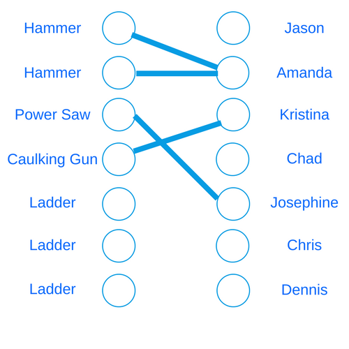
So at this point, are we condemned to choose between a fast inaccurate algorithm and a correct but slow one? In this case the answer is no! This problem is actually best solved by using a graph algorithm! This is an example of what’s called a “bipartite matching” problem. We’ll create a graph with two sets of nodes. On the left, we’ll have a node for each tool. On the right, we’ll have a node for each person. The only edges in our graph will go from nodes on the left towards nodes on the right. A “tool” node has an edge to a “person” node if that person can use the tool. Here’s a partial representation of our graph (plus or minus my design skills). We’ve only drawn in the edges related to Amanda, Christine and Josephine so far.

Now we want to find the “maximum matching” in this graph. That is, we want the largest set of edges such that no two edges share a node. The way to solve this problem using graph algorithms is to turn it into yet ANOTHER graph problem! We’ll add a node on the far left, called the “source” node. We’ll connect it to every “tool” node. Now we’ll add a node on the far right, called the “sink” node. It will receive an edge from every “person” node. All the edges in this graph have a distance of 1.

Again, most of the middle edges are missing here.

The size of the maximum matching in this case is equal to the “max flow” from the source node to the sink node. This is a somewhat advanced concept. But imagine there is water gushing out of the source node and that every edge is a “pipe” whose value (1) is the capacity. We want the largest amount of water that can go through to the sink at once.

Last week we saw built-in functions for shortest path and min spanning tree. FGL also has an out-of-the-box solution for max flow. So our main goal now is to take our objects and construct the above graph.

Preparing Our Solution

A couple weeks ago, we created a segment tree that was very specific to the problem. This time, we’ll show what it’s like to write a more generic algorithm. Throughout the rest of the article, you can imagine that a is a tool, and b is a person. We’ll write a general maxMatching function that will take a list of a’s, a list of b’s, AND a predicate function. This function will determine whether an a object and a b object should have an edge between them. We’ll use the containsTool function from above as our predicate. Then we'll call our general function.

findMaxMatchingBest :: [String] -> [(String, [String])] -> Int
findMaxMatchingBest tools personMap = findMaxMatching containsTool tools personMap

…(different module)

findMaxMatching :: (a -> b -> Bool) -> [a] -> [b] -> Int
findMaxMatching predicate as bs = ...

Building Our Graph

To build our graph, we’ll have to decide on our labels. Once again, we’ll only label our edges with integers. In fact, they’ll all have a “capacity” label of 1. But our nodes will be a little more complicated. We’ll want to associate the node with the object, and we have a heterogeneous (and polymorphic) set of items. We’ll make this NodeLabel type that could refer to any of the four types of nodes:

data NodeLabel a b = 
  LeftNode a |
  RightNode b |
  SourceNode |
  SinkNode

Next we’ll start building our graph by constructing the inner part. We’ll make the two sets of nodes as well as the edges connecting them. We’ll assign the left nodes to the indices from 1 up through the size of that list. And then the right nodes will take on the indices from one above the first list's size through the sum of the list sizes.

createInnerGraph 
  :: (a -> b -> Bool) 
  -> [a]
  -> [b]
  -> ([LNode (NodeLabel a b)], [LNode (NodeLabel a b)], [LEdge Int])
createInnerGraph predicate as bs = ...
  where
    sz_a = length as
    sz_b = length bs
    aNodes = zip [1..sz_a] (LeftNode <$> as)
    bNodes = zip [(sz_a + 1)..(sz_a + sz_b)] (RightNode <$> bs)

Next we’ll also make tuples matching the index to the item itself without its node label wrapper. This will allow us to call the predicate on these items. We’ll then get all the edges out by using a list comprehension. We'll pull each pairing and determining if the predicate holds. If it does, we’ll add the edge.

where
  ...
  indexedAs = zip [1..sz_a] as
  indexedBs = zip [(sz_a + 1)..(sz_a + sz_b)] bs
  nodesAreConnected (_, aItem) (_, bItem) = predicate aItem bItem
  edges = [(fst aN, fst bN, 1) | aN <- indexedAs, bN <- indexedBs, nodesAreConnected aN bN]

Now we’ve got all our pieces, so we combine them to complete the definition:

createInnerGraph predicate as bs = (aNodes, bNodes, edges)

Now we’ll construct the “total graph”. This will include the source and sink nodes. It will include the indices of these nodes in the return value so that we can use them in our algorithm:

totalGraph :: (a -> b -> Bool) -> [a] -> [b] 
  -> (Gr (NodeLabel a b) Int, Int, Int)

Now we’ll start our definition by getting all the pieces out of the inner graph as well as the size of each list. Then we’ll assign the index for the source and sink to be the numbers after these combined sizes. We’ll also make the nodes themselves and give them the proper labels.

totalGraph predicate as bs = ...
  where
    sz_a = length as
    sz_b = length bs
    (leftNodes, rightNodes, middleEdges) = createInnerGraph predicate as bs
    sourceIndex = sz_a + sz_b + 1
    sinkIndex = sz_a + sz_b + 2
    sourceNode = (sourceIndex, SourceNode)
    sinkNode = (sinkIndex, SinkNode)

Now to finish this definition, we’ll first create edges from the source out to the right nodes. Then we'll make edges from the left nodes to the sink. We’ll also use list comprehensions there. Then we’ll combine all our nodes and edges into two lists.

where
  ...
  sourceEdges = [(sourceIndex, lIndex, 1) | lIndex <- fst <$> leftNodes]
  sinkEdges = [(rIndex, sinkIndex, 1) | rIndex <- fst <$> rightNodes]
  allNodes = sourceNode : sinkNode : (leftNodes ++ rightNodes)
  allEdges = sourceEdges ++ middleEdges ++ sinkEdges

Finally, we’ll complete the definition by making our graph. As we noted, we'll also return the source and sink indices:

totalGraph predicate as bs = (mkGraph allNodes allEdges, sourceIndex, sinkIndex)
  where
    ...

The Grand Finale

OK one last step! We can now fill in our findMaxMatching function. We’ll first get the necessary components from building the graph. Then we’ll call the maxFlow function. This works out of the box, just like sp and msTree from the last article!

import Data.Graph.Inductive.Graph (LNode, LEdge, mkGraph)
import Data.Graph.Inductive.PatriciaTree (Gr)
import Data.Graph.Inductive.Query.MaxFlow (maxFlow)

findMaxMatching :: (a -> b -> Bool) -> [a] -> [b] -> Int
findMaxMatching predicate as bs = maxFlow graph source sink
  where
    (graph, source, sink) = totalGraph predicate as bs

And we’re done! This will always give us the correct answer and it runs very fast! Take a look at the code on Github if you want to experiment with it!

Conclusion

Whew algorithms are exhausting aren’t they? That was a ton of code we just wrote. Let’s do a quick review. So this time around we looked at an actual problem that was not an obvious graph problem. We even tried a couple different algorithmic approaches. They both had issues though. Ultimately, we found that a graph algorithm was the solution, and we were able to implement it with FGL.

If you want to use FGL (or most any awesome Haskell library), it would help a ton if you learned how to use Stack! This great tool wraps project organization and package management into one tool. Check out our FREE Stack mini-course and learn more!

If you’ve never programmed in Haskell at all, then what are you waiting for? It’s super fun! You should download our Getting Started Checklist for some tips and resources on starting out!

Stay tuned next week for more on the Monday Morning Haskell Blog!