Graphing it Out

In the last two articles we dealt with some algorithmic issues. We were only able to solve these by improving the data structures in our code. First we used Haskell's built in array type for fast indexing. Then when we needed a segment tree, and we decided to make it from scratch. But we can’t roll our own data structure for every problem we encounter. So it’s good to have some systems we can use for more of these advanced topics.

One of the most important categories of data structures we’ll need for algorithms is graphs. Graphs are quite powerful when it comes to representing complicated problems. They are very useful for expressing relationships between data points. In this article, we'll see two types of graph problems. We’ll learn all about a library called the Functional Graph Library (FGL) that is available on Hackage for us to use. We’ll then take a stab at constructing graphs using the library. Finally, we’ll see how simple it is to solve these algorithms using this library once we’ve made our graphs.

For a complete set of the code that we’ll use in this article, check out this Github repository. It’ll show you how you can use Stack to bring the Functional graph library into your code.

If you’ve never used Stack before, it’s an indispensible tool for creating programs in Haskell. You should try out our Stack mini-course and learn more about it.

Graphs 101

For those of you who aren’t familiar with graphs and graph algorithms, I’ll explain a few of the basics here. If you’re very familiar with these already, you can skip this section. A graph contains a series of objects and encodes various relationships between these objects. For each object in our set, we have a “node” in our graph. These are like data points. Then to represent every relationship, we create an “edge” between two different nodes. We often give some kind of value to this edge as a piece of information about the relationship. In this article, we’ll imagine our nodes as places on a map, with the edges representing legal routes between locations. The label of each edge is the distance.

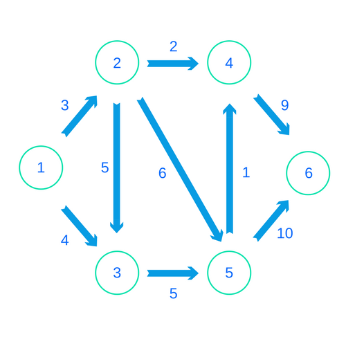
Edges can be both “directed” and “undirected”. Directed edges describe a 1-way relationship between the nodes. Undirected edges describe a 2-way relationship. Here's an example of a graph with directed edges:

Making Graphs with FGL

So whenever we’re making a graph with FGL, we’ll use a two-step process. First, we’ll create the “nodes” of our graph. Then we’ll encode the edges. Let’s suppose we’re reading an input stream. The stream will first give us the number of nodes and then edges in our graph. Then we’ll read a bunch of 3-tuples line-by-line. The first two numbers will refer to the "from" node and the "to" node. The third number will represent the distance. Here’s what this stream might look like for the graph pictured above:

6
9
1 2 3
1 3 4
2 3 5
2 4 2
2 5 6
3 5 5
4 6 9
5 4 1
5 6 10

We’ll read this input stream like so:

import Control.Monad (replicateM)
import System.IO (Handle, hGetLine)

data EdgeSpec = EdgeSpec
  { fromNode :: Int
  , toNode :: Int
  , distance :: Int
  }

readInputs :: Handle -> IO (Int, [EdgeSpec])
readInputs handle = do
  numNodes <- read <$> hGetLine handle
  numEdges <- (read <$> hGetLine handle)
  edges <- replicateM numEdges (readEdge handle)
  return (numNodes, edges)

readEdge :: Handle -> IO EdgeSpec
readEdge handle = do
  input <- hGetLine handle
  let [f_s, t_s, d_s] = words input
  return $ EdgeSpec (read f_s) (read t_s) (read d_s)

Our goal will be to encode this graph in the format of FGL. In this library, every node has an integer identifier. Nodes can either be “labeled” or “unlabeled”. This label, if it exists, is separate from the integer identifier. The function we’ll use requires our nodes to have labels, but we won’t need this extra information. So we’ll use a newtype to wrap the same integer identifier.

Once we know the number of nodes, it’s actually quite easy to create them all. We'll make labels from every number from 1 up through the length. Then we represent each node by the tuple of its index and label. Let’s start a function for creating our graph:

import Data.Graph.Inductive.Graph (mkGraph)
import Data.Graph.Inductive.PatriciaTree (Gr)

…

newtype NodeLabel = NodeLabel Int 
type Distance = Int

genGraph :: (Int, [EdgeSpec]) -> Gr NodeLabel Distance
genGraph (numNodes, edgeSpecs) = mkGraph nodes edges
  where
    nodes = (\i -> (i, NodeLabel i)) 
      <$> [1..numNodes]
    edges = ...

The graph we're making uses a "Patricia Tree" encoding under the hood. We won't go into details about that. We'll just call a simple mkGraph function exposed by the library. We'll make our return value the graph type Gr parameterized by our node label type and our edge label type. As we can see, we’ll use a type synonym Distance for integers to label our edges.

For now let’s get to the business of creating our edges. The format we specified with EdgeSpec works out that we don’t have to do much work. Just as the labeled node type is a synonym for a tuple, the labeled edge is a 3-tuple. It contains the indices of the “from” node, the “to” node, and then the distance label. In this case we’ll use directed edges. We do this for every edge spec, and then we’re done!

genGraph :: (Int, [EdgeSpec]) -> Gr NodeLabel Distance
genGraph (numNodes, edgeSpecs) = mkGraph nodes edges
  where
    nodes = (\i -> (i, NodeLabel i)) 
      <$> [1..numNodes]
    edges = (\es -> (fromNode es, toNode es, distance es))
      <$> edgeSpecs

Using Graph Algorithms

Now suppose we want to solve a particular graph problem. First we’ll tackle shortest path. If we remember from above, the shortest path from node 1 to node 6 on our graph actually just goes along the top, from 1 to 2 to 4 to 6.

How can we solve this from Haskell? We’ll first we’ll use our functions from above to read in the graph. Then we’ll imagine reading in two more numbers for the start and end nodes.

solveSP :: Handle -> IO ()
solveSP handle = do
  inputs <- readInputs handle
  start <- read <$> hGetLine handle
  end <- read <$> hGetLine handle
  let gr = genGraph inputs

Now with FGL we can simply make a couple library calls and we’ll get our results! We’ll use the Query.SP module, which exposes functions to find the shortest path and its length:

import Data.Graph.Inductive.Query.SP (sp, spLength)

solveSP :: Handle -> IO ()
solveSP handle = do
  inputs <- readInputs handle
  start <- read <$> hGetLine handle
  end <- read <$> hGetLine handle
  let gr = genGraph inputs
  print $ sp start end gr
  print $ spLength start end gr

We’ll get our output, which contains a representation of the path as well as the distance. Imagine “input.txt” contains our sample input above, except with two more lines for the start and end nodes “1” and “6”:

>> find-shortest-path < input.txt
[1,2,4,6]
14

We could change our file to instead go from 3 to 6, and then we’d get:

>> find-shortest-path < input2.txt
[3,5,4,6]
15

Cool!

Minimum Spanning Tree

Now let’s imagine a different problem. Suppose our nodes are internet hubs. We only want to make sure they’re all connected to each other somehow. We’re going to pick a subset of the edges that will create a “spanning tree”, connecting all our nodes. Of course, we want to do this in the cheapest way, by using the smallest total “distance” from the edges. This will be our “Minimum Spanning Tree”. First, let’s remove the directions on all the arrows. We can visualize this solution by looking at this picture, and we’ll see that we can connect our nodes at a total cost of 19.

The great news is that it’s not much more work to code this! First, we’ll adjust our graph construction a bit. To have an “undirected” graph in this scenario, we can make our arrows bi-directional like so:

genUndirectedGraph :: (Int, [EdgeSpec]) -> Gr NodeLabel Distance
genUndirectedGraph (numNodes, edgeSpecs) = mkGraph nodes edges
  where
    nodes = (\i -> (i, NodeLabel i)) 
      <$> [1..numNodes]
    edges = concatMap (\es -> 
      [(fromNode es, toNode es, distance es), (toNode es, fromNode es, distance es)])
      edgeSpecs

Besides this, all we have to do now is use the msTree function from the MST module! Then we'll get our result!

import Data.Graph.Inductive.Query.MST (msTree)

...

solveMST :: Handle -> IO ()
solveMST handle = do
  inputs <- readInputs handle
  let gr = genUndirectedGraph inputs
  print $ msTree gr

{- GHC Output
>> find-mst < “input1.txt”
[[(1,0)],[(2,3),(1,0)],[(4,2),(2,3),(1,0)],[(5,1),(4,2),(2,3),(1,0)],[(3,4),(1,0)],[(6,9),(4,2),(2,3),(1,0)]]
-}

This output is a little difficult to interpret, but it’s identical to the tree we saw above. Our output is a list of lists. Each sub-list contains a path from a node to our first node. A path list has a series of tuples, with each tuple corresponding to an edge. The first element of the tuple is the starting node, and the second is the distance.

So the first element, [(1,0)] refers to how node 1 connects to itself, by a single “edge” of distance 0 starting at 1. Then if we look at the last entry, we see node 6 connects to node 1 via a path through nodes 4 and 2, with total distance 9, 2, and 3.

Conclusion

Graph problems are ubiquitous in programming, but it can be a little tricky to get them right. It can be a definite pain to write your own graph data structure from scratch. It can be even harder to write out a full algorithm, even a well known one like Dijkstra's Algorithm. In Haskell, you can use the functional graph library to streamline this process. It has a built in format for representing the graph itself. It can be a little tedious to build up this structure. But once you have it, it’s actually very easy to solve many different common problems.

Next week, we’ll do a bit more work with FGL. We’ll explore a problem that isn’t quite as cut-and-dried as the ones we looked at here. First we'll take a more abstract problem and determine what graph we want to make for it. Then we'll solve that graph problem using FGL. So check back next week on the Monday Morning Haskell blog!.

The easiest way to bring FGL into your Haskell code is to use the Stack tool. If you’re unfamiliar with this, you should take our free Stack mini-course. You’ll learn the important step of how to bring dependencies into your code. You’ll also see the different components in a Stack program and the commands you can run to manipulate them.

If you’ve never programmed in Haskell before, you should try it! Download our Getting Started Checklist. It’ll point you towards some valuable resources in your early Haskell education.