Generalizing Our Environments

In our previous episode, we used Q-Learning to find a solution for the Frozen Lake scenario. We also have a Blackjack game that shares a lot of core ideas with Frozen Lake.
So in this part, we're going to start by applying our Q-Learning solution to the Blackjack game. This will highlight the similarities in the code between the two games. But we'll also see a few differences. The similarities will lead us to create a typeclass for our environment concept. Each "difference" in the two systems will suggest an expression that must be part of the class. Let's explore the implications of this.
Adding to the Environment
Once again, we will need to express our Q-table and the exploration rate as part of the environment. But this time, the index of our Q-Table will need to be a bit more complex. Remember our observation now has three different parts: the user's score, whether the player has an ace, and the dealer's show-card. We can turn each of these into a Word, and combine them with the action itself. This gives us an index with four Word values.
We want to populate this array with bounds to match the highest value in each of those fields.
data BlackjackEnvironment = BlackjackEnvironment
  { ...
  , qTable :: A.Array (Word, Word, Word, Word) Double
  , explorationRate :: Double
  } deriving (Show)

basicEnv :: IO BlackjackEnvironment
basicEnv = do
  gen <- Rand.getStdGen
  let (d, newGen) = shuffledDeck gen
  return $ BlackjackEnvironment
    ...
    (A.listArray ((0,0,0,0), (30, 1, 12, 1)) (repeat 0.0))
    1.0
While we're at it, let's create a function to turn an Observation/Action combination into an index.
makeQIndex :: BlackjackObservation -> BlackjackAction
  -> (Word, Word, Word, Word)
makeQIndex (BlackjackObservation pScore hasAce dealerCard) action =
  ( pScore
  , if hasAce then 1 else 0
  , fromIntegral . fromEnum $ dealerCard
  , fromIntegral . fromEnum $ action
  )
With the help of this function, it's pretty easy to re-use most of our code from last time! The action choice function and the learning function look almost the same! So review last week's article (or the code on Github) for details.
Using the Same Game Loop
With our basic functions out of the way, let's now turn our attention to the game loop and running functions. For the game loop, we don't have anything too complicated. It's a step-by-step process.
- Retrieve the current observation
- Choose the next action
- Use this action to step the environment
- Use our "learning" function to update the Q-Table
- If we're done, return the reward. Otherwise recurse.
Here's what it looks like. Recall that we're taking our action choice function as an input. All our functions live in a similar monad, so this is pretty easy.
gameLoop :: (MonadIO m) =>
  StateT BlackjackEnvironment m BlackjackAction ->
  StateT BlackjackEnvironment m (BlackjackObservation, Double)
gameLoop chooseAction = do
  oldObs <- currentObservation <$> get
  newAction <- chooseAction
  (newObs, reward, done) <- stepEnv newAction
  learnQTable oldObs newObs reward newAction
  if done
    then do
      if reward > 0.0
        then liftIO $ putStrLn "Win"
        else liftIO $ putStrLn "Lose"
      return (newObs, reward)
    else gameLoop chooseAction
Now to produce our final output and run game iterations, we need a little wrapper code. We create (and reset) our initial environment. Then we pass it to an action that runs the game loop and reduces the exploration rate when necessary.
playGame :: IO ()
playGame = do
  env <- basicEnv
  env' <- execStateT resetEnv env
  void $ execStateT stateAction env'
  where
    numEpisodes = 10000
    decayRate = 1.0
    minEpsilon = 0.01

    stateAction :: StateT BlackjackEnvironment IO ()
    stateAction = do
      rewards <- forM [1..numEpisodes] $ \i -> do
        resetEnv
        when (i `mod` 100 == 99) $ do
          bje <- get
          let e = explorationRate bje
          let newE = max minEpsilon (e * decayRate)
          put $ bje { explorationRate = newE }
        (_, reward) <- gameLoop chooseActionQTable
        return reward
      lift $ print (sum rewards)
Now we can play our game! Even with learning, we'll still only get around 40% of the points available. Blackjack is a tricky, luck-based game, so this isn't too surprising.
Constructing a Class
Now if you look very carefully at the above code, it should almost work for Frozen Lake as well! We'd only need to make a few adjustments to naming types. This tells us we have a general structure between our different games. And we can capture that structure with a class.
Let's look at the common elements between our environments. These are all functions we call from the game loop or runner:
- Resetting the environment
- Stepping the environment (with an action)
- Rendering the environment (if necessary)
- Apply some learning method on the new data
- Diminish the exploration rate
So our first attempt at this class might look like this, looking only at the most important fields:
class Environment e where
  resetEnv :: (Monad m) => StateT e m Observation
  stepEnv :: (Monad m) => Action
    -> StateT e m (Observation, Double, Bool)
  renderEnv :: (MonadIO m) => StateT e m ()
  learnEnv :: (Monad m) =>
    Observation -> Observation -> Double -> Action -> StateT e m ()

instance Environment FrozenLakeEnvironment where
  ...

instance Environment BlackjackEnvironment where
  ...
We can make two clear observations about this class. First, we need to generalize the Observation and Action types! These are different in our two games and this isn't reflected above. Second, we're forcing ourselves to use the State monad over our environment. This isn't necessarily wise. It might force us to add extra fields to the environment type that don't belong there.
The solution to the first issue is to make this class a type family! Then we can associate the proper data types for observations and actions. The solution to the second issue is that our class should be over a monad instead of the environment itself.
Remember, a monad provides the context in which a computation takes place. So in our case, our game, with all its stepping and learning, is that context!
Doing this gives us more flexibility for figuring out what data should live in which types. It makes it easier to separate the game's internal state from auxiliary state, like the exploration rate.
Here's our second try, with associated types and a monad.
newtype Reward = Reward Double

class (MonadIO m) => EnvironmentMonad m where
  type Observation m :: *
  type Action m :: *
  resetEnv :: m (Observation m)
  currentObservation :: m (Observation m)
  stepEnv :: (Action m) -> m (Observation m, Reward, Bool)
  renderEnv :: m ()
  learnEnv ::
    (Observation m) -> (Observation m) ->
    Reward -> (Action m) -> m ()
  explorationRate :: m Double
  reduceExploration :: Double -> Double -> m ()
There are a couple undesirable parts of this. Our monad has to be IO to account for rendering. But it's possible for us to play the game without needing to render. In fact, it's also possible for us to play the game without learning!
So we can separate this into more typeclasses! We'll have two "subclasses" of our Environment. We'll make a separate class for rendering. This will be the only class that needs an IO constraint. Then we'll have a class for learning functionality. This will allow us to "run" the game in different contexts and limit the reach of these effects.
newtype Reward = Reward Double

class (Monad m) => EnvironmentMonad m where
  type Observation m :: *
  type Action m :: *
  currentObservation :: m (Observation m)
  resetEnv :: m (Observation m)
  stepEnv :: (Action m) -> m (Observation m, Reward, Bool)

class (MonadIO m, EnvironmentMonad m) =>
  RenderableEnvironment m where
    renderEnv :: m ()

class (EnvironmentMonad m) => LearningEnvironment m where
  learnEnv ::
    (Observation m) -> (Observation m) ->
    Reward -> (Action m) -> m ()
  explorationRate :: m Double
  reduceExploration :: Double -> Double -> m ()
Conclusion
Next week we'll explore how to implement these classes for our different games! We'll end up with a totally generic function for playing the game. We'll have a version with learning and a version without!
The next step after this will be to attach more sophisticated learning mechanisms. Soon, we'll explore how to expand our Q-Learning beyond simple discrete states. The way to do this is to use tensors! So in a couple weeks, we'll explore how to use TensorFlow to construct a function for Q-Learning. To get ready, download our Haskell TensorFlow Guide!
Frozen Lake with Q-Learning!

In the last few weeks, we've written two simple games in Haskell: Frozen Lake and Blackjack. These games are both toy examples from the Open AI Gym. Now that we've written the games, it's time to explore more advanced ways to write agents for them.
In this article, we'll explore the concept of Q-Learning. We've talked about this idea on the MMH blog before. But now we'll see it in action in a simpler context than we did before. We'll write a little bit of Python code, following some examples for Frozen Lake. Then we'll try to implement the same ideas in Haskell. Along the way, we'll see more patterns emerge about our games' interfaces.
We won't be using Tensorflow in the article. But we'll soon explore ways to augment our agent's capabilities with this library! To learn about Haskell and Tensorflow, download our TensorFlow guide!
Making a Q-Table
Let's start by taking a look at this basic Python implementation of Q-Learning for Frozen Lake. This will show us the basic ideas of Q-Learning. We start out by defining a few global parameters, as well as Q, a variable that will hold a table of values.
epsilon = 0.9
min_epsilon = 0.01
decay_rate = 0.9
Total_episodes = 10000
max_steps = 100
learning_rate = 0.81
gamma = 0.96

env = gym.make('FrozenLake-v0')
Q = numpy.zeros((env.observation_space.n, env.action_space.n))
Recall that our environment has an action space and an observation space. For this basic version of the Frozen Lake game, an observation is a discrete integer value from 0 to 15. This represents the location our character is on. Then the action space is an integer from 0 to 3, for each of the four directions we can move. So our "Q-table" will be an array with 16 rows and 4 columns.
How does this help us choose our move? Well, each cell in this table has a score. This score tells us how good a particular move is for a particular observation state. So we could define a choose_action function in a simple way like so:
def choose_action(observation):
  return numpy.argmax(Q[observation, :])
This will look at the different values in the row for this observation, and choose the highest index. So if the "0" value in this row is the highest, we'll return 0, indicating we should move left. If the second value is highest, we'll return 1, indicating a move down.
But we don't want to choose our moves deterministically! Our Q-Table starts out in the "untrained" state. And we need to actually find the goal at least once to start back-propagating rewards into our maze. This means we need to build some kind of exploration into our system. So each turn, we can make a random move with probability epsilon.
def choose_action(observation):
  action = 0
  if np.random.uniform(0, 1) < epsilon:
    action = env.action_space.sample()
  else:
    action = numpy.argmax(Q[observation, :])
  return action
As we learn more, we'll diminish the exploration probability. We'll see this below!
Updating the Table
Now, we also want to be able to update our table. To do this, we'll write a function that follows the Q-learning rule. It will take two observations, the reward for the second observation, and the action we took to get there.
def learn(observation, observation2, reward, action):
  prediction = Q[observation, action]
  target = reward + gamma * numpy.max(Q[observation2, :])
  Q[observation, action] = Q[observation, action] +
                              learning_rate * (target - prediction)
For more details on what happens here, read our Q-Learning primer. But there's one general rule.
Suppose we move from Observation O1 to Observation O2 with action A. We want the Q-table value for the pair (O1, A) to be closer to the best value we can get from O2. And we want to factor in the potential reward we can get by moving to O2. Thus our goal square should have the reward of 1. And squares near it should have values close to this reward!
Playing the Game
Playing the game now is straightforward, following the examples we've done before. We'll have a certain number of episodes. Within each episode, we make our move, and use the reward to "learn" for our Q-table.
for episode in range(total_episodes):
  obs = env.reset()
  t = 0
  if episode % 100 == 99:
    epsilon *= decay_rate
    epsilon = max(epsilon, min_epsilon)

  while t < max_steps:
    action = choose_action(obs)
    obs2, reward, done, info = env.step(action)
    learn(obs, obs2, reward, action)
    obs = obs2
    t += 1

    if done:
      if reward > 0.0:
        print("Win")
      else:
        print("Lose")
      break
Notice also how we drop the exploration rate epsilon every 100 episodes or so. We can run this, and we'll observe that we lose a lot at first. But by the end we're winning more often than not! At the end of the series, it's a good idea to save the Q-table in some sensible way.
Haskell: Adding a Q-Table
To translate this into Haskell, we first need to account for our new pieces of state. Let's extend our environment type to include two more fields. One will be for our Q-table. We'll use an array for this as well, as this gives convenient accessing and updating syntax. The other will be the current exploration rate:
data FrozenLakeEnvironment = FrozenLakeEnvironment
  { ...
  , qTable :: A.Array (Word, Word) Double
  , explorationRate :: Double
  }
Now we'll want to write two primary functions. First, we'll want to choose our action using the Q-Table. Second, we want to be able to update the Q-Table so we can "learn" a good path.
Both of these will use this helper function. It takes an Observation and the current Q-Table and produces the best score we can get from that location. It also provides us the action index. Note the use of a tuple section to produce indices.
maxScore ::
  Observation ->
  A.Array (Word, Word) Double ->
  (Double, (Word, Word))
maxScore obs table = maximum valuesAndIndices
  where
    indices = (obs, ) <$> [0..3]
    valuesAndIndices = (\i -> (table A.! i, i)) <$> indices
Using the Q-Table
Now let's see how we produce our actions using this table. As with most of our state functions, we'll start by retrieving the environment. Then we'll get our first roll to see if this is an exploration turn or not.
chooseActionQTable ::
  (MonadState FrozenLakeEnvironment m) => m Action
chooseActionQTable = do
  fle <- get
  let (exploreRoll, gen') = randomR (0.0, 1.0) (randomGenerator fle)
  if exploreRoll < explorationRate fle
    ...
If we're exploring, we do another random roll to pick an action and replace the generator. Otherwise we'll get the best scoring move and derive the Action from the returned index. In both cases, we use toEnum to turn the number into a proper Action.
chooseActionQTable ::
  (MonadState FrozenLakeEnvironment m) => m Action
chooseActionQTable = do
  fle <- get
  let (exploreRoll, gen') = randomR (0.0, 1.0) (randomGenerator fle)
  if exploreRoll < explorationRate fle
    then do
      let (actionRoll, gen'') = Rand.randomR (0, 3) gen'
      put $ fle { randomGenerator = gen'' }
      return (toEnum actionRoll)
    else do
      let maxIndex = snd $ snd $
                       maxScore (currentObservation fle) (qTable fle)
      put $ fle {randomGenerator = gen' }
      return (toEnum (fromIntegral maxIndex))
The last big step is to write our learning function. Remember this takes two observations, a reward, and an action. We start by getting our predicted value for the original observation. That is, what score did we expect when we made this move?
learnQTable :: (MonadState FrozenLakeEnvironment m) =>
  Observation -> Observation -> Double -> Action -> m ()
learnQTable obs1 obs2 reward action = do
  fle <- get
  let q = qTable fle
      actionIndex = fromIntegral . fromEnum $ action
      prediction = q A.! (obs1, actionIndex)
  ...
Now we specify our target. This combines the reward (if any) and the greatest score we can get from our new observed state. We use these values to get a newValue, which we put into the Q-Table at the original index. Then we put the new table into our state.
learnQTable :: (MonadState FrozenLakeEnvironment m) =>
  Observation -> Observation -> Double -> Action -> m ()
learnQTable obs1 obs2 reward action = do
  fle <- get
  let q = qTable fle
      actionIndex = fromIntegral . fromEnum $ action
      prediction = q A.! (obs1, actionIndex)
      target = reward + gamma * (fst $ maxScore obs2 q)
      newValue = prediction + learningRate * (target - prediction)
      newQ = q A.// [((obs1, actionIndex), newValue)]
  put $ fle { qTable = newQ }
  where
    gamma = 0.96
    learningRate = 0.81
And just like that, we're pretty much done! We can slide these new functions right into our existing functions!
Conclusion
The rest of the code is straightforward enough. We make a couple tweaks as necessary to our gameLoop so that it actually calls our training function. Then we just update the exploration rate at appropriate intervals. Take a look at our code our Github for more details! This week's code is in FrozenLake2.hs.
We've now got an agent that can play Frozen Lake coherently using Q-Learning! Next time, we'll try to adopt this agent for Blackjack as well. We'll see the similarities between the two games. Then we'll start formulating some ideas to combine the approaches.
Blackjack: Following the Patterns

For a couple weeks now, we've been exploring the basics of Open AI Gym. The Frozen Lake example has been our basic tool so far, and we've now written it in Haskell. We'd like to start training agents for this game soon. But first, we want to make sure we're set up to generalize our idea of an environment.
So this week, we're going to make another small example game. This time, we'll play Blackjack. This will give us an example of an environment that needs a more complex observation state. When we're done with this example, we'll be able to compare our two examples. The end goal is to be able to use the same code to train an algorithm for either of them.
If you want to dive into machine learning, you'll need to understand TensorFlow first! Read this guide to learn how to use TensorFlow with Haskell!
Basic Rules
If you don't know the basic rules of casino blackjack, take a look here. Essentially, we have a deck of cards, and each card has a value. We want to get as high a score as we can without exceeding 21 (a "bust"). Each turn, we want to either "hit" and add another card to our hand, or "stand" and take the value we have.
After we get all our cards, the dealer must then draw cards under specific rules. The dealer must "hit" until their score is 17 or higher, and then "stand". If the dealer busts or our score beats the dealer, we win. If the scores are the same it's a "push".
Here's a basic Card type we'll work with to represent the card values, as well as their scores.
data Card =
  Two | Three | Four | Five |
  Six | Seven | Eight | Nine |
  Ten | Jack | Queen | King | Ace
  deriving (Show, Eq, Enum)

cardScore :: Card -> Word
cardScore Two = 2
cardScore Three = 3
cardScore Four = 4
cardScore Five = 5
cardScore Six = 6
cardScore Seven = 7
cardScore Eight = 8
cardScore Nine = 9
cardScore Ten = 10
cardScore Jack = 10
cardScore Queen = 10
cardScore King = 10
cardScore Ace = 1
The Ace can count as 1 or 11. We account for this in our scoring functions:
-- Returns the base sum, as well as a boolean if we have
-- a "usable" Ace.
baseScore :: [Card] -> (Word, Bool)
baseScore cards = (score, score <= 11 && Ace `elem` cards)
  where
    score = sum (cardScore <$> cards)

scoreHand :: [Card] -> Word
scoreHand cards = if hasUsableAce then score + 10 else score
  where
    (score, hasUsableAce) = baseScore cards
Core Environment Types
As in Frozen Lake, we need to define types for our environment. The "action" type is straightforward, giving only two options for "hit" and "stand":
data BlackjackAction = Hit | Stand
  deriving (Show, Eq, Enum)
Our observation is more complex than in Frozen Lake. We have more information that can guide us than just knowing our location. We'll boil it down to three elements. First, we need to know our own score. Second, we need to know if we have an Ace. This isn't clear from the score, and it can give us more options. Last, we need to know what card the dealer is showing.
data BlackjackObservation = BlackjackObservation
  { playerScore :: Word
  , playerHasAce :: Bool
  , dealerCardShowing :: Card
  } deriving (Show)
Now for our environment, we'll once again store the "current observation" as one of its fields.
data BlackjackEnvironment = BlackjackEnvironment
  { currentObservation :: BlackjackObservation
  ...
  }
The main fields are about the cards in play. We'll have a list of cards for our own hand. Then we'll have the main deck to draw from. The dealer's cards will be a 3-tuple. The first is the "showing" card. The second is the hidden card. And the third is a list for extra cards the dealer draws later.
data BlackjackEnvironment = BlackjackEnvironment
  { currentObservation :: BlackjackObservation
  , playerHand :: [Card]
  , deck :: [Card]
  , dealerHand :: (Card, Card, [Card])
  ...
  }
The last pieces of this will be a boolean for whether the player has "stood", and a random generator. The boolean helps us render the game, and the generator helps us reset and shuffle without using IO.
data BlackjackEnvironment = BlackjackEnvironment
  { currentObservation :: BlackjackObservation
  , playerHand :: [Card]
  , deck :: [Card]
  , dealerHand :: (Card, Card, [Card])
  , randomGenerator :: Rand.StdGen
  , playerHasStood :: Bool
  } deriving (Show)
Now we can use these to write our main game functions. As in Frozen Lake, we'll want functions to render the environment and reset it. We won't go over those in this article. But we will focus on the core step function.
Playing the Game
Our step function starts out simply enough. We retrieve our environment and analyze the action we get.
stepEnv :: (Monad m) => BlackjackAction ->
  StateT BlackjackEnvironment m (BlackjackObservation, Double, Bool)
stepEnv action = do
  bje <- get
  case action of
    Stand -> ...
    Hit -> ...
Below, we'll write a function to play the dealer's hand. So for the Stand branch, we'll update the state variable for the player standing, and call that helper.
stepEnv action = do
  bje <- get
  case action of
    Stand -> do
      put $ bje { playerHasStood = True }
      playOutDealerHand
    Hit -> ...
When we hit, we need to determine the top card in the deck. We'll add this to our hand to get the new player score. All this information goes into our new observation, and the new state of the game.
stepEnv action = do
  bje <- get
  case action of
    Stand -> ...
    Hit -> do
      let (topCard : remainingDeck) = deck bje
          pHand = playerHand bje
          currentObs = currentObservation bje
          newPlayerHand = topCard : pHand
          newScore = scoreHand newPlayerHand
          newObservation = currentObs
            { playerScore = newScore
            , playerHasAce = playerHasAce currentObs ||
                             topCard == Ace}
      put $ bje { currentObservation = newObservation
                , playerHand = newPlayerHand
                , deck = remainingDeck }
      ...
Now we need to analyze the player's score. If it's greater than 21, we've busted. We return a reward of 0.0 and we're done. If it's exactly 21, we'll treat that like a "stand" and play out the dealer. Otherwise, we'll continue by returning False.
stepEnv action = do
  bje <- get
  case action of
    Stand -> ...
    Hit -> do
      ...
      if newScore > 21
        then return (newObservation, 0.0, True)
        else if newScore == 21
          then playOutDealerHand
          else return (newObservation, 0.0, False)
Playing out the Dealer
To wrap up the game, we need to give cards to the dealer until their score is high enough. So let's start by getting the environment and scoring the dealer's current hand.
playOutDealerHand :: (Monad m) =>
  StateT BlackjackEnvironment m (BlackjackObservation, Double, Bool)
playOutDealerHand = do
  bje <- get
  let (showCard, hiddenCard, restCards) = dealerHand bje
      currentDealerScore = scoreHand (showCard : hiddenCard : restCards)
If the dealer's score is less than 17, we can draw the top card, add it to their hand, and recurse.
playOutDealerHand :: (Monad m) => StateT BlackjackEnvironment m (BlackjackObservation, Double, Bool)
playOutDealerHand = do
  ...
  if currentDealerScore < 17
    then do
      let (topCard : remainingDeck) = deck bje
      put $ bje { dealerHand =
                    (showCard, hiddenCard, topCard : restCards)
                , deck = remainingDeck}
      playOutDealerHand
    else ...
Now all that's left is analyzing the end conditions. We'll score the player's hand and compare it to the dealer's. If the dealer has busted, or the player has the better score, we'll give a reward of 1.0. If they're the same, the reward is 0.5. Otherwise, the player loses. In all cases, we return the current observation and True as our "done" variable.
playOutDealerHand :: (Monad m) => StateT BlackjackEnvironment m (BlackjackObservation, Double, Bool)
playOutDealerHand = do
  bje <- get
  let (showCard, hiddenCard, restCards) = dealerHand bje
      currentDealerScore = scoreHand
        (showCard : hiddenCard : restCards)
  if currentDealerScore < 17
    then ...
    else do
      let playerScore = scoreHand (playerHand bje)
          currentObs = currentObservation bje
      if playerScore > currentDealerScore || currentDealerScore > 21
        then return (currentObs, 1.0, True)
        else if playerScore == currentDealerScore
          then return (currentObs, 0.5, True)
          else return (currentObs, 0.0, True)
Odds and Ends
We'll also need code for running a loop and playing the game. But that code though looks very similar to what we used for Frozen Lake. This is a promising sign for our hopes to generalize this with a type class. Here's a sample playthrough of the game. As inputs, 0 means "hit" and 1 means "stand".
So in this first game, we start with a King and 9, and see the dealer has a 6 showing. We "stand", and the dealer busts.
6 X

K 9
19 # Our current score
1   # Stand command

1.0 # Reward
Episode Finished

6 9 8 # Dealer's final hand
23  # Dealer's final (busted) score

K 9
19
In this next example, we try to hit on 13, since the dealer has an Ace. We bust, and lose the game.
A X

3 J
13
0

0.0
Episode Finished

A X

K 3 J
23
Conclusion
Of course, there are a few ways we could make this more complicated. We could do iterated blackjack to allow card-counting. Or we could add advanced moves like splitting and doubling down. But that's not necessary for our purposes. The main point is that we have two fully functional games we can work with!
Next time, we'll start digging into the machine learning process. We'll see what techniques we can use with the Open Gym in Python and start translating those to Haskell.
We left out quite a bit of code in this example, particularly around setup. Take a look at our Github repository to see all the details!
Frozen Lake in Haskell

Last time on MMH, we began our investigation into Open AI Gym. We started by using the Frozen Lake toy example to learn about environments. An environment is a basic wrapper that has a specific API for manipulating the game.
Last week's work was mostly in Python. But this week, we're going to do a deep dive into Haskell and consider how to write the Frozen Lake example. We'll see all the crucial functions from the Environment API as well as how to play the game. Take a look at our Github repository to see any extra details about this code!
This process will culminate with training agents to complete these games with machine learning. This will involve TensorFlow. So if you haven't already, download our Haskell Tensor Flow Guide. It will teach you how to get the framework up and running on your machine.
Core Types
In the previous part, we started defining our environment with generic values. For example, we included the action space and observation space. For now, we're actually going to make things more specific to the Frozen Lake problem. This will keep our example much simpler for now. In the coming weeks, we'll start examining how to generalize the idea of an environment and spaces.
We need to start with the core types of our application. We'll begin with a TileType for our board, as well as observations and actions.
data TileType =
  Start |
  Goal |
  Frozen |
  Hole
  deriving (Show, Eq)

type Observation = Word

data Action =
  MoveLeft |
  MoveDown |
  MoveRight |
  MoveUp
  deriving (Show, Eq, Enum)
As in Python, each observation will be a single number indicating where we are on the board. We'll have four different actions. The Enum instance will help us convert between these constructors and numbers.
Now let's consider the different elements we actually need within the environment. The game's main information is the grid of tiles. We'll store this as an Array. The indices will be our observation values, and the elements will be the TileType. For convenience, we'll also store the dimensions of our grid:
data FrozenLakeEnvironment = FrozenLakeEnvironment
  { grid :: Array Word TileType
  , dimens :: (Word, Word) -- Rows, Columns
  ...
  }
We also need some more information. We need the current player location, an Observation. We'll want to know the previous action, for rendering purposes. The game also stores the chance of slipping each turn. The last piece of state we want is the random generator. Storing this within our environment lets us write our step function in a pure way, without IO.
data FrozenLakeEnvironment = FrozenLakeEnvironment
  { grid :: Array Word TileType
  , dimens :: (Word, Word) -- Rows, Cols
  , currentObservation :: Observation
  , previousAction :: Maybe Action
  , slipChance :: Double
  , randomGenerator :: Rand.StdGen
  }
API Functions
Now our environment needs its API functions. We had three main ones last time. These were reset, render, and step. Last week we wrote these to take the environment as an explicit parameter. But this time, we'll write them in the State monad. This will make it much easier to chain these actions together later. Let's start with reset, the simplest function. All it does is set the observation as 0 and remove any previous action.
resetEnv :: (Monad m) => StateT FrozenLakeEnvironment m Observation
resetEnv = do
  let initialObservation = 0
  fle <- get
  put $ fle { currentObservation = initialObservation
            , previousAction = Nothing }
  return initialObservation
Rendering is a bit more complicated. When resetting, we can use any underlying monad. But to render, we'll insist that the monad allows IO, so we can print to console. First, we get our environment and pull some key values out of it. We want the current observation and each row of the grid.
renderEnv :: (MonadIO m) => StateT FrozenLakeEnvironment m ()
renderEnv = do
  fle <- get
  let currentObs = currentObservation fle
      elements = A.assocs (grid fle)
      numCols = fromIntegral . snd . dimens $ fle
      rows = chunksOf numCols elements
  ...
We use chunksOf with the number of columns to divide our grid into rows. Each element of each row-list is the pairing of the "index" with the tile type. We keep the index so we can compare it to the current observation. Now we'll write a helper to render each of these rows. We'll have another helper to print a character for each tile type. But we'll print X for the current location.
renderEnv :: (MonadIO m) => StateT FrozenLakeEnvironment m ()
renderEnv = do
  ...
  where
    renderRow currentObs row = do
      forM_ row (\(idx, t) -> liftIO $ if idx == currentObs
        then liftIO $ putChar 'X'
        else liftIO $ putChar (tileToChar t))
      putChar '\n'

tileToChar :: TileType -> Char
...
Then we just need to print a line for the previous action, and render each row:
renderEnv :: (MonadIO m) => StateT FrozenLakeEnvironment m ()
renderEnv = do
  fle <- get
  let currentObs = currentObservation fle
      elements = A.assocs (grid fle)
      numCols = fromIntegral . snd . dimens $ fle
      rows = chunksOf numCols elements
  liftIO $ do
    putStrLn $ case (previousAction fle) of
      Nothing -> ""
      Just a -> "    " ++ show a
    forM_ rows (renderRow currentObs)
  where
    renderRow = ...
Stepping
Now let's see how we update our environment! This will also be in our State monad (without any IO constraint). It will return a 3-tuple with our new observation, a "reward", and a boolean for if we finished. Once again we start by gathering some useful values.
stepEnv :: (Monad m) => Action
  -> StateT FrozenLakeEnvironment m (Observation, Double, Bool)
stepEnv act = do
  fle <- get
  let currentObs = currentObservation fle
  let (slipRoll, gen') = Rand.randomR (0.0, 1.0) (randomGenerator fle)
  let allLegalMoves = legalMoves currentObs (dimens fle)
  let (randomMoveIndex, finalGen) =
          randomR (0, length AllLegalMoves - 1) gen'
  ...

-- Get all the actions we can do, given the current observation
-- and the number of rows and columns
legalMoves :: Observation -> (Word, Word) -> [Action]
...
We now have two random values. The first is for our "slip roll". We can compare this with the game's slipChance to determine if we try the player's move or a random move. If we need to do a random move, we'll use randomMoveIndex to figure out which random move we'll do.
The only other check we need to make is if the player's move is "legal". If it's not we'll stand still. The applyMoveUnbounded function tells us what the next Observation should be for the move. For example, we add 1 for moving right, or subtract 1 for moving left.
stepEnv :: (Monad m) => Action
  -> StateT FrozenLakeEnvironment m (Observation, Double, Bool)
stepEnv act = do
  ...
  let newObservation = if slipRoll >= slipChance fle
        then if act `elem` allLegalMoves
          then applyMoveUnbounded
                  act currentObs (snd . dimens $ fle)
          else currentObs
        else applyMoveUnbounded
               (allLegalMoves !! nextIndex)
               currentObs
               (snd . dimens $ fle)
  ...

applyMoveUnbounded ::
  Action -> Observation -> Word -> Observation
...
To wrap things up we have to figure out the consequences of this move. If it lands us on the goal tile, we're done and we get a reward! If we hit a hole, the game is over but our reward is 0. Otherwise there's no reward and the game isn't over. We put all our new state data into our environment and return the necessary values.
stepEnv :: (Monad m) => Action
  -> StateT FrozenLakeEnvironment m (Observation, Double, Bool)
stepEnv act = do
  ...
  let (done, reward) = case (grid fle) A.! newObservation of
        Goal -> (True, 1.0)
        Hole -> (True, 0.0)
        _ -> (False, 0.0)
  put $ fle { currentObservation = newObservation
            , randomGenerator = finalGen
            , previousAction = Just act }
  return (newObservation, reward, done)
Playing the Game
One last step! We want to be able to play our game by creating a gameLoop. The final result of our loop will be the last observation and the game's reward. As an argument, we'll pass an expression that can generate an action. We'll give two options. One for reading a line from the user, and another for selecting randomly. Notice the use of toEnum, so we're entering numbers 0-3.
gameLoop :: (MonadIO m) =>
  StateT FrozenLakeEnvironment m Action ->
  StateT FrozenLakeEnvironment m (Observation, Double)
gameLoop chooseAction = do
  ...

chooseActionUser :: (MonadIO m) => m Action
chooseActionUser = (toEnum . read) <$> (liftIO getLine)

chooseActionRandom :: (MonadIO m) => m Action
chooseActionRandom = toEnum <$> liftIO (Rand.randomRIO (0, 3))
Within each stage of the loop, we render the environment, generate a new action, and step the game. Then if we're done, we return the results. Otherwise, recurse. The power of the state monad makes this function quite simple!
gameLoop :: (MonadIO m) =>
  StateT FrozenLakeEnvironment m Action ->
  StateT FrozenLakeEnvironment m (Observation, Double)
gameLoop chooseAction = do
  renderEnv
  newAction <- chooseAction
  (newObs, reward, done) <- stepEnv newAction
  if done
    then do
      liftIO $ print reward
      liftIO $ putStrLn "Episode Finished"
      renderEnv
      return (newObs, reward)
    else gameLoop chooseAction
And now to play our game, we start with a simple environment and execute our loop!
basicEnv :: IO FrozenLakeEnvironment
basicEnv = do
  gen <- Rand.getStdGen
  return $ FrozenLakeEnvironment
    { currentObservation = 0
    , grid = A.listArray (0, 15) (charToTile <$> "SFFFFHFHFFFHHFFG")
    , slipChance = 0.0
    , randomGenerator = gen
    , previousAction = Nothing
    , dimens = (4, 4)
    }

playGame :: IO ()
playGame = do
  env <- basicEnv
  void $ execStateT (gameLoop chooseActionUser) env
Conclusion
This example illustrates two main lessons. First, the state monad is very powerful for managing any type of game situation. Second, defining our API makes implementation straightforward. Next week, we'll explore another toy example with a different state space. This will lead us on the path to generalizing our data structure.
Remember, if you need any more details about these code samples, take a look at the full code on Github! You should also subscribe to Monday Morning Haskell! You'll get our monthly newsletter and access to our subscriber resources!
Open AI Primer: Frozen Lake!

Last year, we spent quite a bit of time on this blog creating a game using the Gloss library. This process culminated in trying to use machine learning to train an agent to play our Maze Game well. The results were not particularly successful. But I've always wanted to come back to the idea of reinforcement learning for game agents.
The Open AI Gym is an open source project for teaching the basics of reinforcement learning. It provides a framework for understanding how we can make agents that evolve and learn. It's written in Python, so this first article will be mostly in Python. But we can (and will) try to implement many of the ideas in Haskell. This week, we'll start exploring some of the core concepts. We'll examine what exactly an "environment" is and how we can generalize the concept. In time, we'll also see how Gloss can help us.
We'll ultimately use machine learning to train our agents. So you'll want some guidance on how to do that in Haskell. Read our Machine Learning Series and download our Tensor Flow guide to learn more!
Frozen Lake
To start out our discussion of AI and games, let's go over the basic rules of one of the simplest examples, Frozen Lake. In this game, our agent controls a character that is moving on a 2D "frozen lake", trying to reach a goal square. Aside from the start square ("S") and the goal zone ("G"), each square is either a frozen tile ("F") or a hole in the lake ("H"). We want to avoid the holes, moving only on the frozen tiles. Here's a sample layout:
SFFF
FHFH
FFFH
HFFG
So a safe path would be to move down twice, move right twice, down again, and then right again. What complicates the matter is that tiles can be "slippery". So each turn, there's a chance we won't complete our move, and will instead move to a random neighboring tile.
Playing the Game
Now let's see what it looks like for us to actually play the game using the normal Python code. This will get us familiar with the main ideas of an environment. We start by "making" the environment and setting up a loop where the user can enter their input move each turn:
import gym
env = gym.make('FrozenLake-v0')
env.reset()

while True:
  move = input("Please enter a move:")
  ...
There are several functions we can call on the environment to see it in action. First, we'll render it, even before making our move. This lets us see what is going on in our console. Then we have to step the environment using our move. The step function makes our move and provides us with 4 outputs. The primary ones we're concerned with are the "done" value and the "reward". These will tell us if the game is over, and if we won.
while True:
  env.render()
  move = input("Please enter a move:")
  action = int(move)
  observation, reward, done, info = env.step(action)
  if done:
    print(reward)
    print("Episode finished")
    env.render()
    break
We use numbers in our moves, which our program converts into the input space for the game. (0 = Left, 1 = Down, 2 = Right, 3 = Up).
We can also play the game automatically, for several iterations. We'll select random moves by using action_space.sample(). We'll discuss what the action space is in the next part. We can also use reset on our environment at the end of each iteration to return the game to its initial state.
for i in range(20):
  observation = env.reset()
  for t in range(100):
    env.render()
    print(observation)
    action = env.action_space.sample()
    observation, reward, done, info = env.step(action)
    if done:
      print("Episode finished after {} timesteps".format(t + 1))
      break

env.close()
These are the basics of the game. Let's go over some of the details of how an environment works, so we can start imagining how it will work in Haskell.
Observation and Action Spaces
The first thing to understand about environments is that each environment has an "observation" space and an "action" space. The observation space gives us a numerical representation of the state of the game. This doesn't include the actual layout of our board, just the mutable state. For our frozen lake example, this is only the player's current position. We could use two numbers for the player's row and column. But in fact we use a single number, the row number multiplied by the column number.
Here's an example where we print the observation after moving right twice, and then down. We have to call reset before using an environment. Then calling this function gives us an observation we can print. Then, after each step, the first return value is the new observation.
import gym
env = gym.make('FrozenLake-v0')
o = env.reset()
print(o)
o, _, _, _ = env.step(2)
print(o)
o, _, _, _ = env.step(2)
print(o)
o, _, _, _ = env.step(1)
print(o)


# Console output
0
1
2
6
So, with a 4x4 grid, we start out at position 0. Then moving right increases our position index by 1, and moving down increases it by 4.
This particular environment uses a "discrete" environment space of size 16. So the state of the game is just a number from 0 to 15, indicating where our agent is. More complicated games will naturally have more complicated state spaces.
The "action space" is also discrete. We have four possible moves, so our different actions are the integers from 0 to 3.
import gym
env = gym.make('FrozenLake-v0')
print(env.observation_space)
print(env.action_space)

# Console Output
Discrete(16)
Discrete(4)
The observation space and the action space are important features of our game. They dictate the inputs and outputs of the each game move. On each turn, we take a particular observation as input, and produce an action as output. If we can do this in a numerical way, then we'll ultimately be able to machine-learn the program.
Towards Haskell
Now we can start thinking about how to represent an environment in Haskell. Let's think about the key functions and attributes we used when playing the game.
- Observation space
- Action space
- Reset
- Step
- Render
How would we represent these in Haskell? To start, we can make a type for the different numeric spaces can have. For now we'll provide a discrete space option and a continuous space option.
data NumericSpace =
  Discrete Int |
  Continuous Float
Now we can make an Environment type with fields for these spaces. We'll give it parameters for the observation type and the action type.
data Environment obs act = Environment
  { observationSpace :: NumericSpace
  , actionSpace :: NumericSpace
  ...
  }
We don't know yet all the rest of the data our environment will hold. But we can start thinking about certain functions for it. Resetting will take our environment and return a new environment and an observation. Rendering will be an IO action.
resetEnv :: Environment obs act -> (obs, Environment obs act)

renderEnv :: Environment obs act -> IO ()
The step function is the most important. In Python, this returns a 4-tuple. We don't care about the 4th "info" element there yet. But we do care to return our environment type itself, since we're in a functional language. So we'll return a different kind of 4-tuple.
stepEnv :: Environment obs act -> act
  -> (obs, Float, Bool, Environment obs act)
It's also possible we'll use the state monad here instead, as that could be cleaner. Now this isn't the whole environment obviously! We'd need to store plenty of unique internal state. But what we see here is the start of a typeclass that we'll be able to generalize across different games. We'll see how this idea develops!
Conclusion
Hopefully you've got a basic idea now of what makes up an environment we can run. Next time, we'll push a bit further with our Haskell and implement Frozen Lake there!
Adding Interactivity with Elm!

A couple weeks ago, we learned how we could serve HTML code from a Haskell server using Servant. Doing this without a system like Reflex left us with a quandry. We still want interactivity on our web pages. But we'd like to do this in a functional way, without writing a lot of Javascript.
Reflex FRP is only one of several options for writing frontend code in a functional language. A while back we considered how to do this with Elm. In this final part of our series, we'll combine Servant with Elm to produce an interactive page.
There are, of course, other options both for frontend and backend when making web apps. Take a look at our Production Checklist to learn more!
A Basic Counter
For a more in depth look at Elm, you should explore our full series on the topic. But for now, let's go over a quick and simple application that we could put in a browser. This app will have a "model" and we will pass "messages" using UI components.
The model will just be an integer counter. And we'll pass "increment" and "decrement" messages by clicking a couple of buttons. We start an Elm application by defining our model and message types. We'll use an alias for the integer model.
type alias Model = Int
type Msg = Increment | Decrement
Now we need to specify how each message type updates our model. An increment message will increase it, and a decrement message will decrease it.
update : Msg -> Model -> Model
update msg model =
  case msg of
    Increment -> model + 1
    Decrement -> model - 1
Next we generate the HTML elements for our page with a view function. This takes our Model and returns Html to display. We'll have two buttons to send the increment and decrement messages. Then we'll also display the current count.
import Html exposing (Html, button, div, text)
import Html.Events exposing (onClick)

view : Model -> Html Msg
view model =
  div []
    [ button [onClick Decrement] [text "-"]
    , div [] [text (String.fromInt model) ]
    , button [onClick Increment] [text "+"]
    ]
Finally, we generate our final application as a "main" expression. We use Browser.sandbox, and pass an initial model value, as well as our update and view expressions.
import Browser

main = Browser.sandbox { init = 0, update = update, view = view}
Compiling Our Elm
Supposing we've written this code in an Elm project as Main.elm, it's now quite easy to compile it into a full HTML file. We run this command:
elm make src/Main.elmThis produces a file index.html that contains our full Elm application. The file requires a lot of boilerplate to get Elm working, so it's over 5000 lines long! But if we return that from our server instead of a blaze-generated HTML file, our app will work!
Referencing Elm
We could make manual modifications to this HTML file to do other things like adding our own CSS. But often times it's easier to compile the Elm into a Javascript file we can include with our other assets. To do this, we just have to tweak our command by outputting to a .js file:
elm make src/Main.elm --output elm.jsThis output file now contains all 5000 lines of our compiled Elm. Now we can make our own HTML file that looks like this:
<html>
  <head>...</head>
  <body>
    <div id="elm"></div>
    <script src="/static/elm.js"/>
    <script>
      var app = Elm.Main.init({node: document.getElementById("elm")});
    </script>
  </body>
</html>
The first script includes our compiled app. The second, shorter script does the work of embedding the app in the preceding div. In this way, we can embed a smaller Elm application in along with other HTML components if we want to. It's much easier to swap out our other assets without having to re-compile our whole frontend!
Of course, for this to work, we have to use the techniques from our earlier article. Our Servant server must serve its static content from a particular directory. This will allow us to include elm.js and any other scripts we make. And then it has to serve our HTML page for the desired endpoints.
Conclusion
You should now have enough tools at your disposal to make a simple web app using only functional tools! Our Real World Haskell Series will give you a good tutorial on some other parts of the stack. If you need any other tools, take a look at our Production Checklist. You can also take a look at all the code for this brief series on Github.
Starting next week, we're going to transition a bit. We've explored the idea of Haskell and machine learning before on this blog. Next time, we'll start looking at some ideas in game AI and agent development. This will set the stage for a combination of Open AI Gym and Haskell code.
Servant Testing Helpers!

We've been looking at Haskell and HTML code for a few weeks now. Last time, we introduced the idea of serving HTML content from a Servant server. Testing any server can be a little tricky. In our Real World Haskell Series, we explored some of the complications in testing such a server.
This week, we're going to look at a couple shortcuts we can take that will make testing our server a little easier. We'll examine some helpers from the Hspec.Wai library, as well as some Quickcheck expressions we can use with Servant.
For more useful Haskell tools, download our Haskell Production Checklist. It goes through a few other libraries you can use besides Servant for your web apps!
Simple Server
Let's start with the same basic user endpoint we had from last time. This takes a User ID, and returns a User if the ID exists in our "database" (an in-memory map for our example).
data User = ...

instance ToJSON User where
  ...

type MyAPI = "users"  :> Capture "uid" Int :> Get '[JSON] (Maybe User)

userHandler :: Int -> Handler (Maybe User)
userHandler uid = return $ M.lookup uid userDB
We've got a server to run this API, which we can use to make an Application.
myServer :: Server MyAPI
myServer = userHandler

myApi :: Proxy MyAPI
myApi = Proxy

myApp :: Application
myApp = serve myApi myServer

runServer :: IO ()
runServer = run 8080 myApp
But, as with any IO action, testing the behavior of this server is tricky. In our earlier article, we had to jump through several hoops to run some tests using the Hspec library. As a pre-condition of the test, we had to start the IO action. Then we had to construct requests using Servant's client functionality. Unwrapping and analyzing the responses was a bit annoying. Finally, we had to ensure we killed the server at the end. Luckily, there's a simpler way to go through this process.
Test Assertions
The HSpec Wai library attempts to simplify this process. As before, we write our tests in conjunction with Hspec syntax. This gives us the opportunity to put more descriptive information into our tests. Even better, we can use simple functions to send network requests to our server.
The expression we'll construct is a normal Spec, so it can fit right in with any other tests we write using Hspec. The key to this process is the with function, which takes our Application as a parameter:
apiSpec :: Spec
apiSpec = with (return myApp) $ do
  ...
The next key is the get combinator. This creates a test assertion we can use within one of our it statements. It takes a string for the "route" of the request we are sending to our server. The simplest assertion we can make is to check the status code of the reply.
apiSpec :: Spec
apiSpec = with (return myApp) $ do
  Describe "GET /users/1" $ do
    it "responds with 200" $ do
      get "users/1" `shouldRespondWith` 200
The assertion statement shouldRespondWith takes a ResponseMatcher type. We can make this matcher in a few different ways. Passing a simple number will make it only worry about the status code. If we pass a string, it will verify that the response body matches that string. Here's how we can verify that we receive a full user string when the user exists, and a "null" result when they don't.
apiSpec :: Spec
apiSpec = with (return myApp) $ do
  describe "GET /users/1" $ do
    it "responds with 200" $ do
      get "/users/1" `shouldRespondWith` 200
    it "responds with a user" $ do
      get "/users/1" `shouldRespondWith`
        "{'email':'james@test.com','age':25,'name':'James','id':1}"
  describe "GET /users/5" $ do
    it "responds with null" $ do
      get "/users/5" `shouldRespondWith` "null"
Unfortunately there don't seem to be great mechanisms for verifying individual fields. You'll have to build any kind of custom matcher from scratch. It's certainly sub-optimal to have to match the JSON string exactly. We can reduce this burden a bit by using the JSON helper library. This let's us specify the object within a quasi-quoter so we don't have to be as precise in specifying the string:
{-# LANGUAGE QuasiQuotes #-}

apiSpec :: Spec
apiSpec = with (return myApp) $ do
  describe "GET /users/1" $ do
    ...
    it "responds with a user" $ do
      get "/users/1" `shouldRespondWith`
        [json|
        {email: "james@test.com", age: 25, name: "James", id: 1}
        |]
So there are definitely areas to improve this library. But it does provide some useful functionality.
Servant Quick Check
Another helpful way to test our API is to incorporate some of the techniques of Quickcheck. The servant-quickcheck library allows us to make blanket assertions about our API . It does this by sending many arbitrary requests to it.
We can actually incorporate these assertions into Hspec code as well. We start with a single assertion and withServantServer:
quickcheckSpec :: Spec
quickcheckSpec =
  it "API has good properties" $
    withServantServer myApi (return myServer) ...
Our key function takes a proxy for our API as well as an action returning our server. The next part is a function taking a "URL" parameter. We'll then use the serverSatisfies argument with our API and some defaultArgs.
quickcheckSpec :: Spec
quickcheckSpec =
  it "API has good properties" $
    withServantServer myApi (return myServer) $ \burl ->
      serverSatisfies myApi burl defaultArgs
        ...
The final piece is to build our actual assertions. We combine these with <%> and need to use mempty as a base. For a simple example, we can test that our endpoint never returns a 500 status code. We can also check that it never takes longer than a second (1e9 nanoseconds). Here's our complete assertion:
quickcheckSpec :: Spec
quickcheckSpec =
  it "API has good properties" $
    withServantServer myApi (return myServer) $ \burl ->
      serverSatisfies myApi burl defaultArgs
        (not500 <%> notLongerThan 1e9 <%> mempty)
Another assertion we can make is that our API only returns full JSON objects. The client code might depend on parsing these, rather than loose strings or some other format. In our case, this will actually fail with our API, because it can return null.
quickcheckSpec :: Spec
quickcheckSpec =
  it "API has good properties" $
    withServantServer myApi (return myServer) $ \burl ->
      serverSatisfies myApi burl defaultArgs
        -- Check JSON as well!
        (onlyJsonObjects <%>
         not500 <%>
         notLongerThan 1000000000 <%>
         mempty)
This suggests we could reconsider how our API works. We could, for example, have it return a 404 instead of a null object if the user doesn't exist. These are some of the simplest functions in the You can take a look at the documentation for a complete listing.
Conclusion
Next week will be our last article on web applications for a little while. We'll explore what it will take to have "functional frontend" code. We'll use Purescript to generate Javascript and use this code within the HTML we send from our server!
Don't forget to subscribe to Monday Morning Haskell! This will give you access to our monthly newsletter as well as our subscriber resources!
Serving HTML with Servant

We now have several different ways of generating HTML code from Haskell. Our last look at this issue explored the Lucid library. But in most cases you won't be writing client side Haskell code.
You'll have to send the HTML you generate to your end-user, typically over a web server. So in this article we're going to explore the most basic way we can do that. We'll see how we can use the Servant library to send HTML in response to API requests.
For a more in-depth tutorial on making a web app with Servant, read our Real World Haskell series! You can also get some more ideas for Haskell libraries in our Production Checklist.
Servant Refresher
Suppose we have a basic User type, along with JSON instances for it:
data User = User
  { userId :: Int
  , userName :: String
  , userEmail :: String
  , userAge :: Int
  }

instance FromJSON User where
  …

instance ToJSON User where
  ...
In Servant, we can expose an endpoint to retrieve a user by their database ID. We would have this type in our API definition, and a handler function.
type MyAPI =
  "users" :> Capture "uid" Int :> Get '[JSON] (Maybe User) :<|>
  ... -- other endpoints

userHandler :: Int -> Handler (Maybe User)
…

myServer :: Server MyAPI
myServer =
  userHandler :<|>
  ... -- Other handlers
Our endpoint says that when we get a request to /users/:uid, we'll return a User object, encoded in JSON. The userHandler performs the logic of retrieving this user from our database.
We would then let client side Javascript code actually to the job of rendering our user as HTML. But let's flip the script a bit and embrace the idea of "server side rendering." Here, we'll gather the user information and generate HTML on our server. Then we'll send the HTML back in reply. First, we'll need a couple pieces of boilerplate.
A New Content Type
In the endpoint above, the type list '[JSON] refers to the content type of our output. Servant knows when we have JSON in our list, it should include a header in the response indicating that it's in JSON.
We now want to make a content type for returning HTML. Servant doesn't have this by default. If we try to return a PlainText HTML string, the browser won't render it! It will display the raw HTML string on a blank page!
So to make this work, we'll start with two types. The first will be HTML. This will be our equivalent to JSON, and it's a dummy type, with no actual data! The second will be RawHtml, a simple wrapper for an HTML bytestring.
import Data.ByteString.Lazy as Lazy

data HTML = HTML

newtype RawHtml = RawHtml { unRaw :: Lazy.ByteString }
We'll use the HTML type in our endpoints as we currently do with JSON. It's a content type, and our responses need to know how to render it. This means making an instance of the Accept class. Using some helpers, we'll make this instance use the content-type: text/html header.
import Network.HTTP.Media ((//), (/:))
import Servant.API (Accept(..))

instance Accept HTML where
  contenType _ = "text" // "html" /: ("charset", "utf-8")
Then, we'll link our RawHtml type to this HTML class with the MimeRender class. We just unwrap the raw bytestring to send in the response.
instance MimeRender HTML RawHtml where
  mimeRender _ = unRaw
This will let us use the combination of HTML content type and RawHtml result type in our endpoints, as we'll see. This is like making a ToJSON instance for a different type to use with the JSON content type.
An HTML Endpoint
Now we can rewrite our endpoint so that it returns HTML instead! First we'll make a function that renders our User. We'll use Lucid in this case:
import Lucid

renderUser :: Maybe User -> Html ()
renderUser maybeUser = html_ $ do
  head_ $ do
    title_ "User Page"
    link_ [rel_ "stylesheet", type_ "text/css", href_ "/styles.css"]
  body_ $ userBody
  where
    userBody = case maybeUser of
      Nothing -> div_ [class_ "login-message"] $ do
        p_ "You aren't logged in!"
        br_ []
        a_ [href_ "/login"] "Please login"
      Just u -> div_ [class_ "user-message"] $ do
        p_ $ toHtml ("Name: " ++ userName u)
        p_ $ toHtml ("Email: " ++ userEmail u)
        p_ $ toHtml ("Age: " ++ show (userAge u))
Now we'll need to re-write our endpoint, so it uses our new type:
type MyAPI = "users" :> Capture "uid" Int :> Get '[HTML] RawHtml :<|>
  ...
Finally, we would rewrite our handler function to render the user immediately!
userHandler :: Int -> Handler RawHtml
userHandler uid = do
  maybeUser <- fetchUser uid -- DB lookup or something
  return (RawHtml $ renderHtml (renderUser maybeUser))
Our server would now work, returning the HTML string, which the browser would render!
Serving Static Files
There's one more thing we need to handle! Remember that HTML by itself is not typically enough. Our HTML files almost always reference other files, like CSS, Javascript, and images. When the user loads the HTML we send, they'll make another immediate request for those files. As is, our server won't render any styles for our user HTML. How do we serve these?
In Servant, the answer is the serveDirectoryWebApp function. This allows us to serve out the files from a particular file as static files. The first piece of this puzzle is to add an extra endpoint to our server definition. This will catch all patterns and return a Raw result. This means the contents of a particular file.
type MyAPI =
  "users" :> Capture "uid" Int :> Get '[HTML] RawHtml :<|>
  Raw
This endpoint must come last out of all our endpoints, even if we compose MyAPI with other API types. Otherwise it will catch every request and prevent other handlers from operating! This is like when you use a catch-all too early in a case statement.
Now for our "handler", we'll use the special serve function.
myServer :: Server MyAPI
myServer =
  userHandler <|>:
  serveDirectoryWebApp "static"
And now, if we have styles.css with appropriate styles, they'll render correctly!
Conclusion
It's a useful exercise to go through the process of making our HTML content type manually. But Blaze and Lucid both have their own helper libraries to simplify this. Take a look at servant-blaze and servant-lucid. You can import the corresponding modules and this will handle the boilerplate for you.
Next week, we'll explore a few extra things we can do with Servant. We'll see some neat combinators that allow us to test our Servant API with ease!
Don't forget you can take a look at our Github repository for more details! This week's code is in `src/BasicServant.hs.
And also remember to subscribe to Monday Morning Haskell! You'll get our monthly newsletter and access to our subscriber resources!
Lucid: Another HTML Option

We're currently looking at different Haskell libraries for generating HTML code. We've already explored how to do this a bit in Reflex FRP and using the Blaze library. This week, we'll consider one more library, Lucid. Then next week we'll start looking at some more complex things we can do with our generated code.
The approaches from Reflex and Blaze have a lot of similarities. In particular, both use monadic composition for building the tree. Lucid will continue this theme as well, and it will generally have a lot in common with Blaze. But there are a few differences as well, and we'll explore those a bit.
If you want to play around with the code from this article a bit more, you should clone our Github repository! This repo contains the simpler Blaze and Html code, as well as some ways we'll use it. If you're ready to work on a full web application, you can also read our Real World Haskell series. This will walk you through the basics of building a web backend with a particular library stack. You can also download our Production Checklist to learn about more options!
Similar Basics
Hopefully, you've already gotten familiar with Blaze's syntax. But even if you're not, we're going to dive straight into Lucid. This syntax is pretty straightforward, as long as you know the basic HTML markup symbols. Here's the input form example we did last time, only now, using Lucid:
{-# LANGUAGE OverloadedStrings #-}

module LucidLib where

import Lucid

mainHtml :: Html ()
mainHtml = html_ $ do
  head_ $ do
    title_ "Random Stuff"
    link_ [rel_ "stylesheet", type_ "text/css", href_ "screen.css"]
  body_ $ do
    h1_ "Welcome to our site!"
    h2_ $ span_ "New user?"
    div_ [class_ "create-user-form"] $ do
      form_ [action_ "createUser"] $ do
        input_ [type_ "text", name_ "username"]
        input_ [type_ "email", name_ "email"]
        input_ [type_ "password", name_ "password"]
        input_ [type_ "submit", name_ "submit"]
    br_ []
    h2_ $ span_ "Returning user?"
    div_ [class_ "login-user-form"] $ do
      form_ [action_ "login"] $ do
        input_ [type_ "email", name_ "email"]
        input_ [type_ "password", name_ "password"]
        input_ [type_ "submit", name_ "submit"]
    br_ []
Right away things look pretty similar. We use a monad to compose our HTML tree. Each new action we add in the monad adds a new item in the tree. Our combinators match the names of HTML elements.
But there are, of course, a few differences. For example, we see lists for attributes instead of using the ! operator. Every combinator and attribute name has underscores. Each of these differences has a reason, as outlined by the author Chris Done in his blog post. Feel free to read this for some more details. Let's go over some of these differences.
Naming Consistency
Let's first consider the underscores in each element name. What's the reason behind this? In a word, the answer is consistency. Let's recall what blaze looks like:
import Text.Blaze.Html5 as H
import Text.Blaze.Html5.Attributes as A

blazeHtml :: Html
blazeHtml = docTypeHtml $ do
  H.head $ do
    H.title "Our web page"
  body $ do
    h1 "Welcome to our site!"
    H.div ! class_ "form" $ do
      p "Hello"
Notice first the qualified imports. Some of the elements conflict with Prelude functions. For example, we use head with normal lists and div for mathematics. Another one, class_, conflicts with a Haskell keyword, so it needs an underscore. Further, we can use certain combinators, like style, either as a combinator or as an attribute. This is why we have two imports at the top of our page. It allows us to use H.style as a combinator or A.style as an attribute.
Just by adding an underscore to every combinator, Lucid simplifies this. We only need one import, Lucid, and we have consistency. Nothing needs qualifying.
Attribute Lists
Another difference is attributes. In Blaze, we used the ! operator to compose attributes. So if we want several attributes on an item, we can keep adding them like so:
-- Blaze
stylesheet :: Html
stylesheet =
  link ! rel "stylesheet" ! href "styles.css" ! type_ "text/css"
Lucid's approach rejects operators. Instead we use a list to describe our different attributes. Here's our style element in Lucid:
-- Lucid
stylesheet :: Html ()
stylesheet =
  link_ [rel_ "stylesheet", type_ "text/css", href_ "screen.css"]
In a lot of ways this syntax is cleaner. It's easier to have lists as extra expressions we can reuse. It's much easier to append a new attribute to a list than to compose a new expression with operators. At least, you're much more likely to get the type signature correct. Ultimately this is a matter of taste.
One reason for Blaze's approach is to avoid empty parameters on a large number of combinators. If a combinator can take a list as a parameter, what do you do if there are no attributes? You either have [] expressions everywhere or you make a whole secondary set of functions.
Lucid gets around this with some clever test machinery. The following two expressions have the same type, even though the first one has no attributes!
aDiv :: Html ()
aDiv = div_ $ p "Hello"

aDiv2 :: Html ()
aDiv2 = div_ [class_ "hello-div"] $ p_ "Hello"
Due to the class Term, we can both have a normal Html element follow our div, or we can list some attributes first. Certain empty combinators like br_ don't fit this pattern as well. They can't have sub-elements, so we need the extra [] parameter, as you can see above. This pattern is also what enables us to use the same style combinator in both situations.
Rendering
There are other details as well. The Monad instance for Html is better defined in Lucid. Lucid's expressions also have a built-in Show instance, which makes simple debugging better.
For Blaze's part, I'll note one advantage comes in the rendering functionality. It has a "pretty print" renderer, that makes the HTML human readable. I wasn't able to find a function to do this from poking around with Lucid. You can render in Lucid like so:
import Lucid

main :: IO ()
main = renderToFile "hello.html" mainHtml

mainHtml :: Html ()
mainHtml = ...
You'll get the proper HTML, but it won't look very appetizing.
Conclusion
So at the end of the day, Blaze and Lucid are more similar than they are different. So the choice is more one of taste. Now, we never want to produce HTML in isolation. We almost always want to serve it out to users of a more complete system. Next week, we'll start looking at some options for using the Servant library to send HTML to our end users.
There are many different pieces to building a web application! For instance, you'll need a server backend and a database! Download our Production Checklist to learn some more libraries you can use for those!
Blaze: Lightweight Html Generation

We've now got a little experience dealing with Haskell and HTML. In our last article we saw how to use some basic combinators within Reflex FRP to generate HTML. But let's take a step back and consider this problem in a simpler light. What if we aren't doing a full Reflex app? What if we just want to generate an HTML string in the context of a totally different application? Suppose we're using some other library to run our backend and want to send some HTML as a raw string. How can we generate this string?
We wouldn't go through the full effort of setting up a Nix application to run GHCJS and Reflex. We would like to do this with a simple Stack application. In the next couple weeks, we'll consider two simple libraries we can use to generate HTML code. This week, we'll look at the Blaze HTML library. Next week we'll consider Lucid. Then after that, we'll investigate how we can serve the HTML we generate from a Servant server.
For some more ideas of production-ready libraries, download our Production Checklist! Try out some other platforms for database management or frontend development!
Basic Combinators
Let's start with the basics. Blaze has a few things in common with the Reflex method of generating HTML data. It also uses a monadic type to produce the HTML tree. In Blaze, this monad is just called Html. Each new action produces a new element node in the tree. Most every basic HTML element has its own function in the library. So we can start our tree with the basic html tag, and then provide a head element as well as a body.
{-# LANGUAGE OverloadedStrings #-}

import Text.Blaze.Html5 as H
Import Text.Blaze.Html5.Attributes as A

basicHtml :: Html
basicHtml = html $ do
  H.head $ do
    H.title "My HTML page"
  body $ do
    h1 "Welcome to our site!"
In some cases, the HTML element names conflict with Haskell library functions. So we use a qualified import with the letter H or A to be more specific.
The above example will produce the following HTML:
<html>
  <head>
    <title>My HTML Page</title>
  </head>
  <body>
    <h1>Welcome to our site!"</h1>
  </body>
</html>
We can get this as a string by using renderHtml from one of a few different modules in the library. For instance the "Pretty" renderer will give the above format, which is more human readable:
import Text.Blaze.Html.Renderer.Pretty

producePage :: String
producePage = renderHtml basicHtml
We can take our simple HTML now and add a few more elements. For instance, we can also add a "doctype" tag at the top, specifying that it is, in fact HTML. This saves us from needing the basic html combinator. We can also do nesting of different elements, such as lists:
basicHtml :: Html
basicHtml = docTypeHtml $ do
    H.head $ do
    H.title "My HTML page"
  body $ do
    h1 "Welcome to our site!"
    "This is just raw text"
    ul $ do
      li "First item"
      li "Second item"
      li "Third item"
One final observation here is that we can use raw strings as a monadic element. We need the OverloadedStrings extension for this to work. This just makes a raw text item in the HTML tree, without any wrapper. See how the raw text appears in our output here:
<!DOCTYPE HTML>

<html>
  <head>
    <title>My HTML Page</title>
  </head>
  <body>
    <h1>Welcome to our site!"</h1>
    This is just raw text
    <ul>
      <li>First item</li>
      <li>Second item</li>
      <li>Third item</li>
    </ul>
  </body>
</html>
Attributes
Now a key component of HTML is, of course, to use attributes with different items. This allows us to customize them with styles and various other properties. For example, when we use an image element, we should provide a "source" file as well as alternate text. We add different attributes to our items with the ! operator. This operator composes so we can add more attributes. Here is an example:
logoImage :: Html
logoImage = img ! src "logo.png" ! alt "The website's logo"

-- HTML

<img src="logo.png" alt="The website's logo"/>
Naturally, we'll want to use CSS with our page. In the head element we can add a stylesheet using a link element. Then we can apply classes to individual components using class_.
styledHtml :: Html
styledHtml = docTypeHtml $ do
  H.head $ do
    link ! rel "stylesheet" ! href "styles.css"
  body $ do
    div ! class_ "style-1" $ do
      "One kind of div"
    div ! class_ "style-2" $ do
      "A second kind of div"
Using Haskell to Populate Types
Now since our Html elements are normal Haskell expressions, we can use any kind of Haskell type as an input. This can turn our elements into functions that depend on normal application data. For example, we can make a list out of different names:
renderNames :: [String] -> Html
renderNames names = do
  "Here are the names"
  ul $ forM_ names (li . toHtml)
We can also take a more complex data structure and use it as an input to our HTML elements. In this example, we'll show a user their points total if we have a User object. But if not, we'll encourage them to login instead.
data User = User
  { userName :: String
  , userPoints :: Int
  }

pointsDisplay :: Maybe User -> Html
pointsDisplay Nothing = a ! href "/login" $ "Please login!"
pointsDisplay (Just (User name points)) = div ! class_ "user-points" $ do
  "Hi "
  toHtml name
  "!"
  br
  "You have "
  toHtml points
  " points!"
This sort of idea is at the heart of "server side rendering", which we'll explore later on in this series.
Making a Form
Here's one final example, where we'll provide two different forms. One for creating a user account, and one for logging in. They each link to separate actions:
multiformPage :: Html
multiformPage = do
  H.head $ do
    H.title "Our Page"
    link ! rel "stylesheet" ! href "styles.css"
  body $ do
    h1 "Welcome to our site!"
    h2 $ H.span "New user?"
    H.div ! class_ "create-user-form" $ do
      H.form ! action "createUser" $ do
        input ! type_ "text" ! name "username"
        input ! type_ "email" ! name "email"
        input ! type_ "password" ! name "password"
        input ! type_ "submit" ! name "submit"
    br
    h2 $ H.span "Returning user?"
    H.div ! class_ "login-user-form" $ do
      H.form ! action "login" $ do
        input ! type_ "email" ! name "email"
        input ! type_ "password" ! name "password"
        input ! type_ "submit" ! name "submit"
As we can see, monadic syntax gives us a very natural way to work with this kind of "tree building" operation.
Conclusion
Now while we've reduced our dependencies from Reflex, this library does have limitations. There's no clear form of Haskell based dynamism. To make our page dynamic, we'd have to include Javascript files along with our generated HTML! And most of us Haskell developers don't want to be writing much Javascript if we can avoid it.
There are still other ways we can use functional means to get the Javascript we want, besides Reflex! We'll explore those a bit later on.
So Blaze has some limitations, but it serves its purpose well. It's a lightweight way of generating HTML in a very intuitive way. Next week, we'll explore another library, Lucid, that has a similar goal.
You can also take a look at our Github repository to see the full code example for this article!
Download our Production Checklist to learn more! If you liked this article, you might want to consider reading our series on Purescript and Elm!
Reflex HTML Basics

Last week we used Nix to create a very simple application using the Reflex FRP framework. This framework uses the paradigm of Functional Reactive Programming to create web pages. It allows us to use functional programming techniques in a problem space with a lot of input and output.
In this week's article, we're going to start explore this framework some more. We'll start getting a feel for the syntax Reflex uses for making different HTML elements. Once we're familiar with these basics, we can compare Reflex with other frontend Haskell tools.
There are several different options you can explore for making these kinds of pages. For some more ideas, download our Production Checklist. This will also suggest some different libraries you can use for your web app's backend!
A Main Function
Let's start out by looking at the code for the very basic page we made last week. It combines a few of the simplest functions we'll need to be familiar with in Reflex.
{-# LANGUAGE OverloadedStrings #-}

module Frontend.Index where

runIndex :: main ()
runIndex = mainWidget $ el "div" $ text "Welcome to Reflex!"
There are three different functions here: mainWidget, el, and text. The mainWidget function is our interface between Reflex types and the IO monad. It functions a bit like a runStateT function, allowing us to turn our page into a normal program we can run. Here is its type signature:
mainWidget :: (forall t. Widget t ()) -> IO ()We provide an input in some kind of a Widget monad and it will convert it to an IO action. The t parameter is one we'll use throughout our type signatures. Reflex FRP will implicitly track a lot of different events on our page over time. This parameter signifies a particular "timeline" of events.
We won't need to get into too much detail about the parameter. There's only one case where different expressions can have different t parameters. This would be if we have multiple Reflex apps at the same time, and we won't get into this case.
There are other main functions we can use. Most likely, we would want to use mainWidgetWithCss for an full project. This takes a CSS string to apply over our page. We'll want to use the embedFile template function here. This converts a provided filepath into the actual CSS ByteString.
mainWidgetWithCss :: ByteString -> (forall t. Widget t()) -> IO ()

runIndex = do
  let cssString = $(embedFile "static/styles.css")
  mainWidgetWithCss cssString $ el "div" $ text "Hello, Reflex!"
Static Elements
The rest of our combinators will have HTML oriented types. We'll start with our two simple combinators, text and el. These are both different kinds of "widgets" we can use.
The first of these is straightforward enough. It takes a string (Text) and produces an element in a DomBuilder monad. The result of this will be a simple text element appearing on our webpage with nothing wrapping it.
text :: (DomBuilder t m) => Text -> m ()So for example if we omitted the use of el above, the HTML for our web page body would look like:
<body>
  Welcome to Reflex!
</body>
The el combinator then provides us with the chance to wrap one HTML element within another. We provide a first argument with a string for the type of element we're wrapping with. Then we give the monadic action for the HTML element within. In the case of our page, we wrap our original text element with a div.
el :: (DomBuilder t m) => Text -> m () -> m ()

runIndex = mainWidget $ el "div" $ text "Welcome to Reflex!"
This produces the following HTML in our body:
<body>
  <div>Welcome to Reflex!</div>
</body>
Now, because an element takes a monad, we can compose more elements within it as deeply as we want. Here's an example with a couple nested lists:
runIndex = mainWidget $ el "div" $ do
  el "p" (text "Two Lists")
  el "ol" $ do
    el "li" (text "Number One")
    el "li" (text "Number Two")
    el "li" (text "Number Three")
  el "ul" $ do
    el "li" (text "First Item")
    el "li" (text "Second Item")
    el "li" (text "Third Item")
Adding Attributes
Of course, there's more to HTML than creating elements. We'll also want to assign properties to our elements to customize their appearance.
One simple way to do this is to use the elAttr combinator instead of el. This allows us to provide a map of attributes and values. Here's an example where we provide the filename, width, and height of an image element. Note that blank is the same as text "", an empty HTML element:
imageElement = elAttr "image"
  ("src" =. "checkmark.jpg" <> "height" =. "300" <> "width" =. "300")
  blank

-- Produced HTML
<img src="checkmark.jpg" height="300" width="300"></img>
Reflex has some specific combinators we can use to build an attribute map. The =. operator combines two elements to create a singleton map. We can append different maps with the monoid operator <>.
In general, we should handle CSS with static files elsewhere. We would create CSS classes that contain many different properties. We can then apply these classes to our HTML elements. The elClass combinator is an easy way to do thing in Reflex.
styledText = elClass "p" "fancy" (text "Hello")

-- Produced HTML
<p class="fancy">Hello</p>
Now we don't need to worry about styling every individual element.
Conclusion
We already have quite a few opportunities available to us to build our page. Still, it was a big hassle to use Nix and Reflex just to write some Html. Next week, we'll start exploring more lightweight options for doing this in Haskell.
For more resources on building Haskell web tools, download our Production Checklist!
Making the Jump to Real World Haskell
Last week, we announced our Practical Haskell course. Enrollments are still open, but not for much longer! They will close at midnight Pacific time on Wednesday, March 11th, only a couple days from now!
I've always hoped to provide content that would help people make the jump from beginners to seasoned Haskell developers. I want to show that Haskell can be useful for "Real World" applications. Those are the main goals of this course. So in this article, I wanted to share some of the mistakes I made when I was trying to make that jump. These are what motivated me to make this course, so I hope you can learn from them.
Package Management is Key
My Haskell career started with a side project, one you can still see on Github. There were some cool things about the project, but my process had several flaws. The first one was that I had no idea how to organize a Haskell project.
My early work involved writing all my code in .hs source files and running manual tests with runghc. Installing dependencies was a mess (I put everything in the global package database). I eventually learned to use Cabal, but without sandboxing. Dependency hell ensued. It was only after months of working through that process that I learned about Stack. Stack made everything easier, but I could have used it from the start!
Don't repeat my mistake! Learn how to use Stack, or just Cabal, or even Nix! This will solve so many of your early problems. It will also streamline the rest of your development process. Speaking of...
Test First, Integrate Completely
When it comes to making a project, the first question you should ask is, "How will my customer use this?" When it comes to writing code within that project, you should always then ask, "How will I know this code works?"
These two questions will guide your development and help avoid unnecessary rework. It's a natural tendency of developers that we want to jump in on the "meat" of the problem. It's exactly the mistake I made on that first project. I just wanted to write Haskell! I didn't want to worry about scripting or package non-sense. But these issues will ultimately get in the way of what you really want to do. So it's worth putting in the effort to overcome them.
The first step of the project as a whole should be to build out your end-to-end pipeline. That is, how will you put this code out there on the web? How will someone end up using your code? There will often be tedious scripting involved, and dealing with services (CI, AWS, etc.). But once that work is out of the way, you can make real progress.
Then when developing a particular component, always know how you'll test it. Most often, this will be through unit testing. But sometimes you'll find it's more complicated than that. Nothing's more frustrating than thinking you're done coding and finding problems later. So it's important to take the time to learn about the frameworks that let you test things with ease. Keep practicing over and over again until testing is second nature.
Start Simple
Another important thing when it comes to the learning process is knowing how to start small. I learned this over the course of my machine learning series last fall. My methods were often so ineffective that I didn't know if the algorithm I was trying to implement worked at all. But the problem I was trying to solve was too difficult! I've found more success in machine learning by starting with simpler problems. This way, you'll know the general approach works, and you can scale up accordingly.
This also makes it much easier to follow the advice above! If your system is large and complicated, the scripting and running process will be harder. You'll have to spend more time getting everything up and running. For a smaller project, this is not so difficult. So you'll get valuable practice at a smaller scale. This will make bigger projects smoother once you get there.
Use Both Documentation and Examples
None of us were born knowing how to write Haskell. The first time you use a library, you won't know the best practices. The documentation can help you. It'll list everything you need, but often a lot more. It can be hard to know what's necessary and what's not.
So another great thing to do when starting out is to find a project that has used the library before. You need to establish some baseline of "something that works". This way, you'll have a more solid foundation to build on. You'll have specific examples to work from, which will help build your "end-to-end experience".
In my first project, I used the Parsec library without using any examples! My code was sloppy and repetitive. There were many shortcuts I didn't know about hiding in the docs. And I could have avoided that if I had first looked for a project that also used the library. Then I could have started from there and built my knowledge.
Documentation and examples work in tandem with each other. If you use the docs without examples, you'll miss a lot of shortcuts and practical uses. If you use examples without the docs, you'll miss the broader picture of what else you can do! So both are necessary to your development as a programmer.
Conclusion
Haskell has developed a lot in the last few years, so this is a great time to learn what the language is capable of! Our Practical Haskell course aims to help you become a more seasoned developer. It'll help you avoid all the mistakes I outlined in this article. So if you've got the basics down and want to learn more, this is your chance!
And if you're not as confident in your skills yet, you can also check out our Beginners course! It requires no experience and will walk you through the basics!
Announcing Practical Haskell!

This week we have an exciting announcement! One of the biggest goals of this blog has been to show Haskell's utility as a production language. Our Practical Haskell course is the culmination of that goal. It assumes you have a decent grounding in Haskell basics, including things like monads and using Stack. To sign up, head over to the course page!
Course Overview
The course consists of five modules. Each module has a series of video lectures and accompanying exercises. There are also "screencast" videos where you get to see the techniques from the lectures in action.
Throughout the course, you'll be building a small web application. In the first module, you'll learn how to store the necessary data for this app. We'll take an in-depth look at Persistent, a Haskell database library. This will show us some of the unique features Haskell can bring to this area.
In module 2, we'll learn how to build a web server that provides an API for accessing our database. We'll see how to write endpoints using the Servant library and how we can test those endpoints. We'll also deploy our application using Heroku.
Module 3 provides a frontend for our app. This frontend will be in Elm, rather than Haskell! These languages have very similar syntax. So you'll learn some special libraries and techniques for integrating them. This way, you'll be able to display all the data you're serving!
The fourth module will teach you some advanced ideas for organizing your code. We'll take a deep dive into monad transformers and also learn about free monads!
We'll wrap up the course with an overview of testing in Haskell. We'll start with some common unit testing libraries and work our way up to more advanced techniques.
Besides the course material, there will also be a Slack group for this course. This will be a place where you can get help from myself or any of your fellow classmates!
Course Schedule
The course will launch on Monday, March 16th, with the release of module 1. We will then release a new module each Monday thereafter. Don't worry if you're busy on a particular week! There's no time limit on doing the material. You'll be able to access the content indefinitely.
Sign-ups for the course will end on Wednesday, March 11th! So don't miss out! Head over to the course page and reserve your spot today!
Building a Reflex FRP Project with Nix!
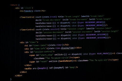
Over these last few weeks, we've gone over a few different package managers we can use with Haskell. Of these, Nix has the broadest potential, but it's also the most complicated to use. This week, we'll conclude our look at package management by putting Nix to work. We'll be using Reflex FRP, a Haskell framework for frontend web development.
This framework has many complicated dependencies, so it's basically necessary to use Nix. Stack and Cabal by themselves aren't going to be able to capture all the requirements. In this article, we'll go through some steps to set ourselves up to make a Reflex FRP project. Along the way, we'll learn a little bit about the basics of this library.
If you're ready for Nix and FRP frontend apps, you're ready to use Haskell for many cool things! Download our Production Checklist for some more ideas!
Project Setup
Before you do this setup phase, take note that it will take quite a while due to the volume of packages. We'll be following along with this guide. You'll want to make a new directory with access to the reflex-platform Git repository.
>> mkdir ReflexProject && cd ReflexProject
>> git init
>> git submodule add https://github.com/reflex-frp/reflex-platform
You then need to run the try-reflex script within that repository. If you don't have Nix, this will install Nix. But regardless, it will then use Nix to install many dependencies needed for Reflex. So feel free to run the command and let your terminal sit for a while.
Managing Multiple Packages
For this project, we'll be using a combination of Nix and Cabal, but in a different way than we tried a couple weeks ago. Back then, we converted a .cabal file to a Nix project. For Reflex FRP, the recommended project structure is to use three different packages. First we would want one for frontend web elements. The second is for a backend server, while we'd have a third common package for elements used by both. To reflect this structure you'll make three different directories. Then run cabal init in each of them.
>> mkdir common frontend backend
>> (cd common && cabal init)
>> (cd frontend && cabal init)
>> (cd backend && cabal init)
The common package will be a library and you should ensure it exposes at least one module. The other two packages should be executables that depend on common. All three should depend on reflex-dom.
Now we need to make a default.nix file to pull this all together. It should look like this:
{ system ? builtins.currentSystem }:
(import ./reflex-platform { inherit system; }).project ({ pkgs, ... }: {
  packages = {
    common = ./common;
    backend = ./backend;
    frontend = ./frontend;
  };

  shells = {
    ghc = ["common" "backend" "frontend"];
    ghcjs = ["common" "frontend"];
  };
})
The simplest part to see is that we list each of our different packages within this expression. Then we declare two "shells" for the different compilers we can use. We can compile any of our 3 packages with GHC. But then for our frontend and its common dependency, we also have the option of using GHCJS. We'll see this come into play in a little bit.
The important thing to notice at the top is that we are using the reflex-platform submodule as a dependency. This lets us avoid worrying about a lot of other dependencies in this file.
A Simple Frontend
Now let's take a step back from our project structure for a second and write out a basic frontend landing page. This code will go in frontend/Main.hs:
{-# LANGUAGE OverloadedStrings #-}

module Main where

import Reflex.Dom

main :: IO ()
main = mainWidget $ el "div" $ text "Welcome to Reflex!"
The Reflex.Dom module exports most of the different elements we'll need to build a simple web page. The mainWidget expression provides us with a way to run a widget as an IO action. Then el allows us to make an element of the specified type (a div in this case). We can then provide some simple text using the text element. As you can probably tell, this will give us a webpage that displays our desired text.
We'll definitely explore more details about Reflex FRP syntax at a later date. But for now, the important thing to understand is that we have a Haskell executable that displays a webpage.
Building Our Code with Nix
But how do actually use this executable? Well there are a couple ways. The first way uses Nix by itself:
>> nix-build -o frontend-result -A ghcjs.frontendNote how we're using the ghcjs shell to compile this instead of ghc. GHCJS knows how to generate Javascript from Haskell, rather than a raw binary.
We can then look in the output directory, frontend-result/bin to see the results. There's another directory frontend.jsexe in there. It contains several Javascript helper files, but one main index.html file. If we pull this index file into our browser, we'll see our web page text!
Building with Cabal
Relying on Nix for building does have a weakness though. Nix doesn't do incremental builds. So it will need to build our whole package every time. This can be frustrating if you like re-building many times after small changes.
So we can also build our frontend with Cabal, which knows how to do things in a more incremental way! We'll still use a nix-shell to ensure we have our all our dependencies.
>> nix-shell -A shells.ghcjs --run \
  "cabal --project-file=cabal-ghcjs.project \
    --builddir=dist-ghcjs new-build all"
Note how we use the GHCJS project to again ensure we get the right output. This will also build our code, producing the same frontend.jsexe directory. This time though, it will live within dist-ghcjs.
A small price of using Cabal is that we have to dig deeper in the file structure to find it (eight directories)! But scripting can relieve this burden. The point is, we can now incrementally build our frontend executable!
Conclusion
This concludes our series on package management! You should now have the tools to get started with some pretty interesting projects. You can use any of the different programs we've covered here, whether Cabal, Stack, Nix, or a combination!
This marks a nice transition point for us. From here we'll move on and look at some interesting concepts when it comes to web development. We'll stick with the general app structure we started building here with Reflex FRP. It will be a little while before we look at frontend concepts in earnest though. We'll start by exploring more backend considerations next week.
The coming weeks' topics will be more related to Haskell in production! Download our Production Checklist for more ideas to try!
Using Nix to Fetch C Libraries!

In the last couple weeks, we've started getting our feet wet with the Nix package manager. Last time we used cabal2nix to convert a purely Cabal project into a Nix project. This demonstrated how we could get our Haskell dependencies from the Nix store if we wanted.
But one of the virtues of Nix is that it has much more to it than Haskell packages! Sometimes, we might be using a package that has a trickier dependency, like a C library. We can't capture these in our Stack or Cabal files all that well. Nix however, can install these dependencies as easily as Haskell packages!
This week, we'll see a couple simple ways Nix can do this. The first will be a simple addition to our Nix file. But the second will be more of a hybrid integration with Stack! We'll get our Haskell dependencies from Stack, but others from Nix! It's actually a very simple process!
Nix is a more advanced system for managing our projects. But for some more basic knowledge, you should download our Beginners Checklist. This will acquaint you with some more basic tools to get started with. You can also read our Liftoff Series for a more detailed walkthrough!
Using a C Library
Let's suppose we're doing some task with Linear Programming in Haskell. The GNU Linear Programming Kit (GLPK) is a useful tool for this task. And if we want to interact with the kit through Haskell, we'd want to use the glpk-hs library. If we create a new Stack project, we can add it as a dependency in our .cabal file. We'll also need the package and one of its dependencies as extra-deps in stack.yaml:
extra-deps:
  - glpk-hs-0.7
  - gasp-1.2.0.0
When we do stack build, it will appear to download the packages fine, but then we'll get a strange error:
Missing dependency on a foreign library:
* Missing (or bad) C library: glpk
The Haskell GLPK library uses the C library as a dependency for running some of its tasks. So if we don't have this library installed, we can't proceed. And unfortunately, our normal ways of using Stack don't let us install C libraries.
The normal solution to this would be to download the C library, compile it, and install it. But this is a tedious process. The more dependencies like this you have, the harder it is for anyone to use your library. They'll have a lot more steps involved in setting themselves up to use it or contribute. And it can be difficult to replicate all these same steps on a remote server machine. This can make continuous integration and deployment more painful.
Nix to the Rescue!
While Stack and Cabal aren't great with C libraries, Nix handles them perfectly well! If you take a look at the source repository for glpk-hs, you can read the default.nix file. There's a line in there specifying the C dependency on glpk! Instead of going in the libraryHaskellDepends section, we have a new line. The librarySystemDepends field tells us the system packages our library depends on.
{ ... }:
mkDerivation {
  ...
  libraryHaskellDepends = [array base containers deepseq gasp mtl];
  librarySystemDepends = [glpk];
  ...
}
As long as a user of this code has Nix, all they have to do is nix-build release.nix, and they'll get this C library! It doesn't matter if they're on their own machine or a remote server!
Using Stack and Nix
Using librarySystemDepends is one way of adding system dependencies. But, this workflow forces us to use Nix for our Haskell dependencies as well. To make our little GLPK project work we would make a full nix file with glpk-hs as a Haskell dependency and glpk as a system dependency.
What if we want to use Stack for our Haskell packages and Nix for external packages like C libraries? There's a way to do this with Stack! It's actually quite simple. We'll have our stack.yaml file set up as we did before. Then we'll add these lines to it:
nix:
  enable: true
  packages: [glpk]
By including a nix section with enable: true, Stack knows we want to use Nix. We can then list the system packages we want to retrieve. If we use this approach, our project will build without needing any extra work for glpk.
As another example, suppose we want to use the snappy compression library. But once again, including this package as an extra-dep won't give you the required C library. But if you also include it via Nix, then everything will work!
-- stack.yaml

nix:
  enable: true
  packages: [snappy]

extra-deps:
  - snappy-0.2.0.2
The Stack/Nix combination works by running Stack commands within a nix-shell. So there are some other fields we can add to the nix section that can customize the behavior of this. For example nix-shell-options allows us to pass other options to the command. The path field allows us to specify a specific Nix path. And instead of providing a packages list, we can also provide a full nix-shell file. This gives us the chance to add more configurations if we want.
Conclusion
That's how simple it can be to use Stack with Nix! Next week, we'll wrap up our study of Nix and package managers by exploring how to use GHCJS! This is an awesome Haskell project that lets us compile our Haskell into Javascript to use in web pages. You need to know the basics of Nix before trying it out though!
Appendix: Haskell and Tensor Flow!
If you've read our Machine Learning Series you know how irritating C dependencies can be. Following our Haskell TensorFlow guide involves installing 3 separate C libraries! Hopefully I'll soon be able to provide a guide with an alternative Nix-based approach. It depends on whether Nix has the right versions of the various libraries!
Converting Cabal to Nix!

In last week's article we discussed the basics of the Nix package manager. Nix brings some of the ideas of functional purity to package management in Haskell. For example, when you download a package, there are no side effects on other packages in your system. And any package is a direct product of its dependencies and source code, generating a unique hash.
But Nix doesn't typically work in a standalone fashion with Haskell projects. Like Stack, it actually integrates with Cabal under the hood. We'll continue to use a .cabal file to describe our package. But a neat tool allows us to get the advantages of Nix in conjunction with Cabal. This week, we'll explore how to make a basic project with this combination.
If you're a beginner to Haskell, you're probably better off starting with Stack, rather than Nix. Read our Liftoff Series to get familiar with the language basics. Then you can take our free Stack mini-course to get acquainted with Stack.
Initializing Our Project with Nix
Last week, we explored the nix-shell command. This allows you to run commands as if you had certain packages installed. So even if our system doesn't have GHC or Cabal installed, we can still run the following command:
>> nix-shell --packages ghc cabal-install --run "cabal init"This will open up a shell where Nix gives us the necessary packages. Then it runs the cabal init package, like we saw in our Cabal tutorial a few weeks back. This gives us a basic Cabal project, which we could build and run using Cabal tools.
Converting to Nix
But instead of doing that, we're going to convert it to a Nix project! There's an excellent resource out there that does this conversion for us. The cabal2nix program can take a Cabal file and convert it into a nix package file. How do we install this program? Well, using Nix of course! We can even skip installing it and run the command through nix-shell. Note how we pass the current directory "." as an input to the command, and pipe the output to our nix file, default.nix.
>> nix-shell --packages cabal2nix --run "cabal2nix ." > default.nixHere's the resulting file:
{ mkDerivation, base, stdenv }:
mkDerivation {
 pname = "MyNixProject";
 version = "0.1.0.0";
 src = ./.;
 isLibrary = false;
 isExecutable = true;
 executableHaskellDepends = [ base ];
 license = "unknown"
 hydraPlatforms = stdenv.lib.platforms.none;
}
This file contains a single expression in the Nix language. The first line contains the three "inputs" to our expression. Of these, base is our only Haskell dependency. Then mkDerivation is a Nix function we can use to make our derivation expression. Finally, there's this stdenv dependency. This is a special input telling Nix we have a standard Linux environment. Nix assumes it has certain things like GCC and Bash.
Then we assign certain parameters in our call to mkDerivation. We provide our package name and version. We also state that it contains an executable and not a library (for now). There's a special field where we list Haskell dependencies. This contains only base for now.
We can't build from this file just yet. Instead, we'll make another file release.nix. This file contains, again, a single Nix expression. We use an imported function haskellPackages.callPackage to call our previous file.
let
 pkgs = import <nixpkgs> { };
in
 pkgs.haskellPackages.callPackage ./default.nix { }
We don't provide any parameters for right now, so we'll leave the empty braces there. For a production project, you would use this file to "pin" the nix packages to a particular channel. But we don't need to do that right now.
We can now build our program using the nix-build command and the new release file:
>> nix-build release.nixBuilding the project puts the results in a result directory at your project root. So we can then run our simple binary!
>> ./result/bin/MyNixProject
Hello, Haskell!
Adding a Dependency
As we have in previous tutorials, let's make this a little more interesting by adding a dependency! We'll once again use the basic split package. We'll make a lastName function in our library like so:
module Lib where

import Data.List.Split (splitOn)

lastName :: String -> String
lastName input = last (splitOn " " input)
Then we'll use this in our executable. Instead of simply printing a message, we'll get the user's name and then print their last name:
module Main where

import Lib (lastName)


main :: IO ()
main = do
 putStrLn "What's your name?"
 input <- getLine
 let lName = lastName input
 putStr "Your last name is: "
 putStrLn lName
We'll need to update our .cabal file from its initial state to include the library and the new dependency. Notice we change the executable name to avoid confusion with the library.
library
 build-depends:
     base >=4.12 && <4.13
   , split == 0.2.3.3
 ...

executable run-nix-project
 build-depends:
     base >=4.12 && <4.13
   , MyNixProject
Now that we've changed our .cabal file, we must run cabal2nix again to re-generate default.nix. We do this with the same nix-shell invocation we used earlier. (It's a good idea to save this command to an alias). Then we can see that default.nix has changed.
{ mkDerivation, base, split, stdenv }:
mkDerivation {
 pname = "MyNixProject";
 version = "0.1.0.0";
 src = ./.;
 isLibrary = true;
 isExecutable = true;
 libraryHaskellDepends = [base split ];
 executableHaskellDepends = [ base ];
 license = "unknown"
 hydraPlatforms = stdenv.lib.platforms.none;
}
The new file reflects the changes to our project. The split package is now an input to our project. So it appears as an "argument" on the first line. We've added a library, so we see that isLibrary has changed to true. There's also a new line for libraryHaskellDepends. It contains the split package we use as a dependency. Now Nix will handle the task of finding the right dependency on our channel!
We can once again build our code using nix. We'll see the different behavior, now under a different executable name!
>> nix-build release.nix
>> ./result/bin/run-nix-project
What's your name?
John Test
Your last name is: Test
Conclusion
This wraps up our first look at making a Haskell project with Nix. We still have Cabal providing a basic description of our package. But Nix actually provides us with the package database. Next week, we'll go into these details a little more, and take it one step further. We'll show how we can use Stack and Nix together to unify all the different package managers we've looked at.
As I've mentioned before, Nix does have a steeper learning curve than our other tools. In particular, there are not as many clear tutorials out there. So I recommend starting out with Stack before learning Nix. You can do this by taking our Stack mini-course.
Given the lack of clear tutorials, I want to highlight a couple resources that helped me write this article. First, the haskell-nix Github repository, written by Gabriel Gonzalez. Second this blog post by Soares Chen. These are good resources if you want to go a bit further with Haskell and Nix.
Nix: Functional Package Management!
In the past few weeks we've gone over the two primary build systems people use for Haskell, Stack and Cabal. These systems are specific to Haskell though. You couldn't, for instance, make a C++ or Node.js project using Cabal. This week though, we're going to discuss Nix, a more broadly applicable package manager.
We could use Nix for a project in virtually any programming language. It tends to attract a disproportionate amount of attention from Haskell developers though. There are a couple reasons for this. First, other languages tend to have more mature tool-chains than Haskell. So there's less of a need to explore alternative solutions like Nix. Second, the authors of Nix describe it as a "pure functional" package manager. So its design and functionality incorporate a lot of ideas that attract Haskellers.
So in this article, we're going to discuss the basics features of Nix. It has a few particular advantages due to its functional nature. We'll also do a crash-course in some of the basic commands. Next week, we'll start exploring some more Haskell-specific tasks with it.
While Nix has a lot of cool features, it also has a steep learning curve. So if you're new to Haskell, I strongly recommend you start out with Stack. Read our Liftoff Series and take our free Stack mini-course to learn more!
Installing and Basic Commands
To start out, let's get Nix installed. This is simple enough on a Linux or MacOS machine. You just need to curl the install script and run it:
bash <(curl https://nixos.org/nix/install)Once you have Nix, you'll install packages from "channels". A channel is a mechanism that allows you to get pre-built binaries and libraries. In some ways, it works like Hackage, but for all kinds of programs. By installing, you'll get a stable default channel.
The primary command you'll use is nix-env. This lets you interact with packages on the channel and on your system. For instance, nix-env -qa will list all the available packages you can install from the channel. To actually install a package, you'll use the -i option (or --install). This command will install a basic GNU "hello" program:
>> nix-env -i hello
...
Installing 'hello-2.10'
>> hello
Hello, world!
You can also uninstall a program with the -e option. If you would rather test out a program without installing it, you can make a nix shell for it! The nix-shell command for will bring up a shell that has the program installed for you:
>> nix-env -e hello
>> hello
No such file or directory
>> nix-shell -p hello
[nix-shell:~]$ hello
Hello, world!

[nix-shell:~]$ exit
These simple commands allow you to download other peoples' packages. But the real fun comes with using Nix to make our own packages. We'll get to that next week!
Windows Compatibility
As the name suggests, Nix's authors designed it around Unix-based operating systems. Thus it doesn't exist for Windows. If you program on a Windows machine, your best bet is to use the Windows Subsystem for Linux (WSL). The other option would be some kind of virtual box, but these will slow you down a lot.
On my machine, I found I needed a bit of a hack to get Nix installed on WSL. Instead of installing normally, I followed the advice in this pull request. When installing, you'll want the following line in a pre-existing /etc/nix/nix.conf file.
use-sqlite-wal = falseYou can do this by hand, or use this command as you install:
>> echo 'use-sqlite-wal = false' | \
  sudo tee -a /etc/nix/nix.conf && sh <(curl https://nixos.org/nix/install)
After doing this, everything should work!
Sandboxing on Steroids
Now let's dig into the functionality of Nix a little more. What does it mean that Nix is a "functional" package manager? Well, first off, our actions shouldn't have "side effects". In the case of package management, this means that we can install a program without impacting any other programs on our machine. It's essentially an extreme form of sandboxing.
When you install Nix, it will create a special /nix/store folder at the root of your system. When you use Nix, all packages you download and build on your machine get their own sub-directory. For example, when we installed hello, we get the following directory:
/nix/store/234v87nsmj70i1592h713i6xidfkqyjw-hello-2.10Notice our package has a special hash associated with it. This is important. We could potentially update our channel to check for a newer version. Then we could install that as well. This could create a directory like so, with a different (hypothetical) hash:
>> nix-env --upgrade hello
>> ls /nix/store
/nix/store/abcd123smj70iqaswe713i6xidfpogjq-hello-2.11
...
But the original version of hello would still be in our store! The update and reinstall would have no effect on it, and it would work as it used to. And if we didn't like the new version, we could roll it back!
nix-env --rollbackInputs and Outputs
Now let's investigate what's going on with those hashes. Each nix package is also "functional" in the sense that it is a function of its particular inputs. That is, every package has some list of dependencies as well as the source code. And we can reproduce the output binary from these inputs in a deterministic way.
The hash we get in front of the package gets constructed from all the different inputs. So if we change the dependencies for our package, we'll get a new hash, since the result could be different. And if we change our source code, our hash should also be different, as we're making a new program.
So when we define our own Nix package, we'll describe its dependencies using the Nix Language. This will include listing the versions and build configurations in a .nix file. This allows us to create a "derivation" of our program. And the real upshot is that this derivation will be the same no matter what machine you're on! Nix will ensure that it downloads all the same dependencies and compiles them in the same way.
Conclusion
Hopefully you've now got a good grounding in the basics of Nix. Next week, we'll start exploring how we can make our own Nix projects. We'll look at combining the powers of Cabal and Nix to create a Haskell project!
Hpack: A Simpler Package Format

In the last few weeks, we've gone through the basics of Cabal and Stack. These are two of the most common package managers for Haskell. Both of these programs help us manage dependencies for our code, and compile it. Both programs use the .cabal file format, as we explored in this article.
But .cabal files have some weaknesses, as we'll explore. Luckily, there's another tool out there called Hpack. With this tool, we'll use a different file format for our project, in a file called package.yaml. We'll run the hpack command, which will read the package file and generate the .cabal file. In this article, we'll explore how this program works.
In our free Stack mini-course, you'll learn how to use Stack as well as Hpack! If you're new to Haskell, you can also read our Liftoff series to brush up on your skills!
Cabal File Issues
One of the first weaknesses with the .cabal file is that it uses its own unique format. It doesn't use something more common like XML, JSON, YAML, or Markdown. So there's a small learning curve when it comes to questions of format. For instance, what are good indentation practices? What is the "correct" way to make a list of things? When are commas necessary, or not? And if, for whatever reason, you want to parse whatever is in your package file, you'll need a custom parser.
When using Hpack, we'll still have a package file, package.yaml. But this file uses a YAML format. So if your previous work has involved YAML files, that knowledge is more transferable. And if you haven't yet, it's likely you will use YAML at some point in the future. Plus every major language can parse YAML with ease.
If you're making a project with many executables and tests, you'll also find your .cabal file has a lot of duplication. You'll need to repeat certain fields for each section. Different executables could have the same GHC options and language extensions. The different sections will also tend to have a lot of dependencies in common
In the rest of this article, we'll see how Hpack solves these problems. But first, we need to get it up and running.
Installing and Using Hpack
The Hpack program is an executable you can get from Stack. Within your project directory, you just need to run this command:
stack install hpackAfter this, you should be able to run the hpack command anywhere on your system. If you run it in any directory containing a package.yaml file, the command will use that to generate the .cabal file. We'll explore this package file format in the next section.
When using Hpack, you generally not commit your .cabal file to the Github repository. Instead, put it in .gitignore. Your README should clarify that users need to run hpack the first time they clone the repository.
As an extra note, Hpack is so well thought of that the default Stack template will include package.yaml in your starter project! This saves you from having to write it from scratch.
Package File
But how is this file organized anyway? Obviously we haven't eliminated the work of writing a package file. We've just moved it from the .cabal file to the package.yaml file. But what does this file look like? Well, it has a very similar structure to the Cabal file. But there are a few simplifications, as we'll see. To start, we have a metadata section at the top which is almost identical to that in the Cabal file.
name: MyHpackProject
version: 0.1.0.0
github: jhb563/MyHpackProject
license: MIT
author: "James Test"
maintainer: "james@test.com"
copyright: "Monday Morning Haskell 2020"

extra-source-files:
  - README.md
These lines get translated almost exactly. Various other fields get default values. One exception is that the github repository name will give us a couple extra links for free in the .cabal file.
-- Generated automatically in MyHpackProject.cabal!
homepage: https://github.com/jhb563/MyHpackProject#readme
bug-reports: https://github.com/jhb563/MyHpackProject/issues

source-repository head
  type: git
  location: https://github.com/jhb563/MyHpackProject
After the metadata, we have a separate section for global items. These include things such as dependencies and GHC options. We write these as top level keys in the YAML. We'll see how these factor into our generated file later!
dependencies:
  - base >=4.9 && <4.10

ghc-options:
  - -Wall
Now we get into individual sections for the different elements of our package. But these sections can be much shorter than they are in the .cabal file! For the library portion, we can get away with only listing the source directory!
library:
  source-dirs: src
This simple description gets translated into the library section of the .cabal file:
library
  exposed-modules:
      Lib
  other-modules:
      Paths_MyHpackProject
  hs-source-dirs:
      src
  build-depends:
      base >=4.9 && <4.10
  default-language: Haskell2010
Note that Paths_XXX is an auto-generated module of sorts. Stack uses it during the build process. This is one of a few different parts of this section that Hpack generates for us.
Executables are a bit different in that we group them all together in a single key. We use the top level key executables and then have a separate sub-key for each different binary. These can have their own dependencies and GHC options.
executables:
  run-project-1:
    main: Run1.hs
    source-dirs: app
    ghc-options:
      - -threaded
    dependencies:
      - MyHpackProject
  run-project-2:
    main: Run2.hs
    source-dirs: app
    dependencies:
      - MyHpackProject
From this, we'll get two different exectuable sections in our .cabal file! Note that these inherit the "global" dependency on base and the GHC option -Wall.
exectuable run-project-1
  main-is: Main.hs
  other-modules:
      Paths_MyHpackProject
  hs-source-dirs:
      app
  build-depends:
      MyHpackProject
    , base >=4.9 && <4.10
  ghc-options: -Wall -threaded
  default-language: Haskell2010

executable run-project-2
  ...
Test suites function in much the same way as executables. You'll just want a separate section tests after your executables.
Module Inference
So far we've saved ourselves from writing a bit of non-intuitive boilerplate. But there are more gains to be had! One annoyance of the .cabal file is that you will see error or warning messages if any of your modules aren't listed. So when you make a new module, you always have to update .cabal!
Hpack fixes this issue for us by inferring the layout of our modules! Notice how we made no mention of the individual modules in package.yaml above. But they still appeared in the .cabal file. If we don't specify, Hpack will search our source directory for all Haskell source files. It will assume they all go under exposed-modules. So even if we have a few more files, everything gets listed with the same basic description of our library.
-- Files in source directory
-- src/Lib.hs
-- src/Parser.hs
-- src/Router.hs
-- src/Internal/Helpers.hs

...
-- Hpack Library Section
library:
  source-dirs: src

-- Cabal File Library Section
library
  exposed-modules:
    , Internal.Helpers
    , Lib
    , Parser
    , Router
  other-modules:
      Paths_MyHpackProject
  ...
Hpack also takes care of alphabetizing our modules!
There are, of course, times when we don't want to expose all our modules. In this case, we can list the modules that should remain as "other" in our package file. The rest still appear under exposed-modules.
-- Package File
library:
  source-dirs: src
  other-modules:
    - Internal.Helpers

-- Cabal File
library
  exposed-modules:
    , Lib
    , Parser
    , Router
  other-modules:
      Internal.Helpers
  ...
If you want the external API to be more limited, you can also explicitly list the exposed modules. Hpack infers that the rest fall under "other".
-- Package File
library:
  source-dirs: src
  exposed-modules:
    - Lib
Remember that you still need to run the hpack command when you add a new module! Otherwise there's no update to the .cabal file. This habit takes a little while to learn but it's still easier than editing the file each time!
Reducing Duplication
There's one more area where we can get some de-duplication of effort. This is in the use of "global" values for dependencies and compiler flags.
Normally, the library, executables and test suites must each list all their dependencies and the options they need. So for example, we might find that all our elements use a particular version of the base and aeson libraries, as well as the -Wall flag.
library
  ghc-options: -Wall
  build-depends:
      base >=4.9 && <4.10
    , aeson
  ...

exectuable run-project-1
  ghc-options: -Wall -threaded
  build-depends:
      MyHpackProject
    , aeson
    , base >=4.9 && <4.10
  ...
With Hpack, we can simplify this by creating global values for these. We'll add dependencies and ghc-options as top level keys in our package file. Then each element can include its own dependencies and options as needed. The following will produce the same .cabal file output as above.
dependencies:
  - base >=4.9 && <4.10
  - aeson

ghc-options:
  - -Wall

library:
  source-dirs: src

executables:
  run-project-1:
    ghc-options:
      - -Wall
    dependencies:
      - MyHpackProject
Conclusion
Hpack isn't a cure-all. We've effectively replaced our .cabal file with the package.yaml file. At the end of the day, we still have to put some effort into our package management process. But Hpack saves a good amount of duplicated and manual work we would need to do if we were using the .cabal file by itself. But you need to remember when to run Hpack! Otherwise it can get frustrating. Whenever you have some event that would alter the .cabal file, you need to re-run the command! Do it whenever you add a new module or build dependency!
Next week, we'll start looking at Nix, another popular package manager among Haskellers!
Nicer Package Organization with Stack!

In last week's article we explored Haskell package management using Cabal. This tool has been around for a while and serves as the backbone for Haskell development even to this day. We explored the basics of this tool, but also noticed a few issues. These issues centered around dependency management, and what happens when package versions conflict.
Nowadays, most Haskell developers prefer the Stack tool to Cabal. Stack still uses many of the features of Cabal, but adds an extra layer, which helps deal with the problems we saw. In this article, we'll do a quick overview of the Stack tool and see how it helps.
For a more in depth look at Stack, you should take our free Stack mini-course . While you're at it, you can also download our Beginner Checklist. This will help ensure you're up to speed with the basics of Haskell.
Creating a Stack Project
Making a new project with Stack is a little more streamlined than with Cabal by itself. To start with, we don't need the extra step of creating our project directory before hand. The stack new command handles creating this directory.
>> stack new MyStackProject
>> cd MyStackProject
By default, Stack will also generate some basic source files for our project. We get a library file in src/Lib.hs, an executable program in app/Main.hs, and a test in test/Spec.hs. It also lists these files in the .cabal file. So if you're newer to using Haskell, it's easier to see how the file works.
You can use different templates to generate different starter files. For example, the servant template will generate boilerplate for a Servant web server project. The .cabal file includes some dependencies for using Servant. Plus, the generated starter code will have a very simple Servant server.
>> stack new MyStackProject servantBasic Commands
As with Cabal, there are a few basic commands we can use to compile and run our Haskell code with Stack. The stack build command will compile our library and executables. Then we can use stack exec with an executable name to run that executable:
stack exec run-project-1
stack exec run-project-2
Finally, we can run stack test to run the different test suites in our project. Certain commands are actually variations on stack build, with different arguments. In these next examples, we run all the tests with --test, and then run a single test suite by name.
>> stack build --test
>> stack build MyStackProject:test:test-suite-1
Stack File
Stack still uses Cabal under the hood, so we still have a .cabal file for describing our package format. But, we also have another package file called stack.yaml. If you look at this file, you'll see some new fields. These fields provide some more information about our project as a whole. This information will help us access dependencies better.
The resolver field tells us which set of packages we're using from Stackage. We'll discuss this more later in the article.
resolver: lts-13.19Then the packages field gives a list of the different packages in our project. Stack allows us to manage multiple packages at once with relative ease compared to Cabal. Each entry in this list refers to a single directory path containing a package. Each individual package has its own .cabal file.
packages:
  - ./project-internal
  - ./project-parser
  - ./project-public
Then we also see a field for extra-deps. This lists dependency packages outside of our current resolver set. By default, it should be empty. Again, we'll explore this a bit later once we understand the concept of resolvers better.
Installing Packages
Besides the basic commands, we can also use stack install. But its functionality is a bit different from cabal install. If we just use stack install by itself, this will "install" the executables for this project on our local path. Then we can run them from any directory on our machine.
>> stack install
...
Copied executables to /home/username/.local/bin/
- run-project-1
- run-project-2
>> cd ..
>> run-project-1
"Hello World!"
This is different from the way we installed dependency packages using cabal install. We could use stack install in a similar way. But this is more for different Haskell programs we want to use. For example, we can install the hlint code linter like so:
stack install hlintBut unlike with vanilla Cabal, it's unnecessary to do this with dependency packages! Using stack build installs dependencies for us! We can add a dependency (say the split package), and build our code without a separate install command!
This is one advantage we get from using Stack, but on its own it still seems small. Let's start looking at the real benefits from Stack when it comes to dependency conflicts.
Cross-Project Conflicts
Recall what happened when using different versions of a package on different projects on our machine. We encountered a conflict, since the global index could only have one version of the package. We solved this with Cabal by using sandboxes. A sandbox ensured that a project had an isolated location for its dependencies. Installing packages on other projects would have no effect on this sandbox.
Stack solves this problem as well by essentially forcing us to use sandboxing. It is the default behavior. Whenever we build our project, Stack will generate the .stack-work directory. This directory contains all our dependencies for the project. It also stores our compiled code and executables.
So with Stack, you don't have to remember if you already initialized the sandbox when running normal commands. You also don't have to worry about deleting the sandbox on accident.
Dependency Conflicts
Sandboxing solves the issue of inter-project dependency conflicts. But what about within a project? Stack's system of resolvers is the solution to these. You'll see a "resolver version" in your stack.yaml file. By default, this will be the latest lts version at the time you make your project. Essentially, a resolver is a set of packages that have no conflicts with each other.
Most Haskell dependencies you use live on the Hackage repository. But Stack adds a further layer with Stackage. A resolver set in Stackage contains many of the most common Haskell libraries out there. But there's only a single version of each. Stack maintainers have curated all the resolver sets. They've exhaustively checked that there are no dependency conflicts between the package versions in the set.
Here's an example. The LTS-14.20 resolver uses version 1.4.6.0 of the aeson library. All packages within the resolver that depend on this library will be compatible with this version.
So if you stick to dependencies within the resolver set, you won't have conflicts! This means you can avoid the manual work of finding compatible versions.
There's another bonus here. Stack will determine the right version of the package for us. So we generally don't need version constraints in our .cabal files. We would just list the dependency and Stack will do the rest.
library
  exposed-modules: Lib
  build-depends:
      base
    , split
  ...
You'll generally want to stick to "long term support" (lts) resolvers. But there are also nightly resolvers if you need more bleeding edge libraries. Each resolver also corresponds to a particular version of GHC. So Stack figures out the proper version of the compiler your project needs. You can also rest assured that Stack will only use dependencies that work for that compiler.
Adding Extra Packages
While it's nice to have the assurance of non-conflicting packages, we still have a problem. What if we need Haskell code that isn't part of the resolver set we're using? We can't expect the Stack curators to think of every package we'll ever need. There's a lot of code on Github we could use. And indeed, even many libraries on Hackage are not in a Stackage resolver set.
We can still import these packages though! This is what the extra-deps field of stack.yaml is there for. We can add entries to this list in a few different formats. Generally, if you provide a name and a version number, Stack will look for this library on Hackage. You can also provide a Github repository, or a URL to download. Here are a couple examples:
extra-deps:
  - snappy-0.2.0.2
  - git: https://github.com/tensorflow/haskell.git
    commit: d741c3ee59a5c9569fb2026bd01c1c8ff22fa7c7
Note that you'll still have to add the package name as a dependency in your .cabal file. You can omit the version number though, as we did with other packages above.
Often, using one package as an "extra dependency" will then require other packages outside the resolver set. Getting all these can be a tedious process. But you can usually use the stack solver command to get the full list of packages (and versions) that you need.
Unfortunately, when you introduce extra dependencies you're no longer guaranteed of avoiding conflicts. But if you do encounter conflicts, you have a clear starting point. It's up to you to figure out a version of the new package you can use that is compatible with your other dependencies. So the manual work is much more limited.
Conclusion
That wraps up our look at Stack and how it solves some of the core problems with using Cabal by itself. Next week, we'll explore the hpack tool, which simplifies the process of making our .cabal file. In a couple weeks, we'll also take a look at the Nix package manager. This is another favorite of Haskell developers!
Using Cabal on its Own

Last week we discussed the format of the .cabal file. This file is a "package description" file, like package.json in a Node.js project. It describes important aspects of our project's different pieces. For instance, it tells us what source files we have for our library, and what packages it depends on.
Of course this file is useless without a package manager program to actually build our code! These days, most Haskell projects use Stack for package management. If you want to jump straight into using Stack, take a look at our free Stack mini-course!
But Stack is actually only a few years old. For much of Haskell's history, Caba was the main package management tool. It's still present under the hood when using Stack, which is why Stack still uses the .cabal file. But we can also use it in a standalone fashion, as Haskell developers did for years. This week, we'll explore what this looks like. We'll encounter the problems that ultimately led to the development of Stack.
If you're still new to the Haskell language, you can also read our Liftoff Series to get a better feel for the basics!
Making a New Project
To create a new project using Cabal, you should first be in a specific directory set aside for the project. Then you can use cabal init -n to create a project. This will auto-generate a .cabal file for you with defaults in all the metadata fields.
>> mkdir MyProject && cd MyProject
>> cabal init -n
>> vim MyProject.cabal
The -n option indicates "non-interactive". You can omit that option and you'll get an interactive command prompt instead. The prompt will walk you through all the fields in the metadata section so you can supply the proper information.
>> mkdir MyProject && cd MyProject
>> cabal init
Package name? [default: MyProject]
Package version? [default: 0.1.0.0]
...
Since you only have to run cabal init once per project, it's a good idea to run through the interactive process. It will ensure you have proper metadata so you don't have to go back and fix it later.
Running this command will generate the .cabal file for you, as well as a couple other files. You'll get ChangeLog.md, a markdown file where you can record important changes. It also generates Setup.hs. You won't need to modify this simple boilerplate file. It will also generate a LICENSE file if you indicated which license you wanted in the prompt.
Basic Commands
Initializing the project will not generate any Haskell source files for you. You'll have to do that yourself. Let's suppose we start with a simple library function in a file src/Lib.hs. We would list this file under our exposed-modules field of our library section. Then we can compile the code there with the cabal build command.
If we update our project to have a single executable run-project, then we can also run it with cabal run. But if our project has multiple executables, this won't work. We'll need to specify the name of the executable.
>> cabal run run-project-1
"Hello World 1!"
>> cabal run run-project-2
"Hello World 2!"
You can also run cabal configure. This will do some system checks to make sure you can actually build the program. For instance, it verifies that you have some version of ghc available. You can also use the command to change this compiler version. It also does some checks on the dependencies of your package.
Adding Dependencies
Speaking of dependencies, let's explore adding one to our project. Let's make our library depend on the split package. Using this library, we can make a lastName function like so:
import Data.List.Split(splitOn)

lastName :: String -> String
lastName inputName = splitOn " " inputName
When we try to build this project using, we'll see that our project can't find the Data.List.Split module...yet. We need to add split as a dependency in our library. To show version constraints, let's suppose we want to use the latest version, 0.2.3.3 at the time of writing.
library:
  build-depends:
      base >=4.9 && <4.10
    , split == 0.2.3.3
  ...
This still isn't quite enough! We actually need to install the split package on our machine first! The cabal install command will download the latest version of the package from hackage and put it in a global package index on our machine.
cabal install splitOnce we've done this, we'll be able to build and run our project!
Conflicting Dependencies
Now, we mentioned that our package gets installed in a "global" index on our machine. If you've worked in software long enough, this might have set off some alarm bells. And indeed, this can cause some problems! We've installed version 0.2.3.3 globally. But what if another project wants a different version? Configuring will give an error like the following:
cabal: Encountered missing dependencies:
split ==0.2.3.2
And in fact it's very tricky to have both of these versions installed in the global index!
Using a Sandbox
The way around this is to sandbox our projects. When we do this, each dependency we get from Hackage will get installed in the project-specific sandbox, rather than a global index. Within our project directory, we can create a sandbox like so:
>> cabal sandbox initNow this project will only look at the sandbox for its dependencies. So we'll see the same messages for the missing module when we try to build. But then we'll be fine when we install packages. We can run this version of the command to install all missing packages.
>> cabal install --only-dependenciesNow our project will build without issue, even with a different version of the package!
Conflicts within a Project
Let's consider another scenario that can introduce version conflicts. Suppose we have two dependencies, package A and package B. Each of these might depend on a third package, C. But package A might depend on version X of package C. And then B might depend on version Y of C. Because we can't have two versions of the package installed, our program won't build!
Sandboxes will prevent these issues from occurring across different projects on our machine. But this scenario is still possible inside a single project! And in this case, we'll have to do a lot more manual work than we bargained for. We'll have to go through the different versions of each package, look at their dependencies, and hope we can find some combination that works. It's a messy, error-prone process.
Next week, we'll see how to solve this issue with Stack!
Conclusion
So we can see now that Cabal can stand on its own. But it has certain weaknesses. Stack's main goal is to solve these weaknesses, particularly around dependency management. Next week, we'll see how this happens!