Running From Enemies!

We've spent a few weeks now refactoring a few things in our game. We made it more performant and examined some related concepts. This week, we're going to get back to adding new features to the game! We'll add some enemies, represented by little squares, to rove around our maze! If they touch our player, we'll have to re-start the level!
In the next couple weeks, we'll make these enemies smarter by giving them a better search strategy. Then later, we'll give ourselves the ability to fight back against the enemies. So there will be interesting trade-offs in features.
Remember we have a Github Repository for this project! You can find all the code for this part can in the part-5 branch! For some other interesting Haskell project ideas, download our Production Checklist!
Organizing
Let's remind ourselves of our process for adding new features. Remember that at the code level, our game has a few main elements:
- The
Worldstate type - The update function
- The drawing function
- The event handler
So to change our game, we should update each of these in turn. Let's start with the changes to our world type. First, it's now possible for us to "lose" the game. So we'll need to expand our GameResult type:
data GameResult = GameInProgress | GameWon | GameLostNow we need to store the enemies. We'll add more data about our enemies as the game develops. So let's make a formal data type and store a list of them in our World. But for right now, all we need to know about them is their current location:
data Enemy = Enemy
  { enemyLocation :: Location
  }

data World = World
  { …
  , worldEnemies :: [Enemy]
  }
Updating The Game
Now that our game contains information about the enemies, let's determine what they do! Enemies won't respond to any input events from the player. Instead, they'll update at a regular interval via our updateFunc. Our first concern will be the game end condition. If the player's current location is one of the enemies locations, we've "lost".
updateFunc :: Float -> World -> World
updateFunc _ w =
  -- Game Win Condition
  | playerLocation w == endLocation w = w { worldResult = GameWon }
  -- Game Loss Condition
  | playerLocation w `elem` (enemyLocation <$> worldEnemies w) =
      w { worldResult = GameLost }
  | otherwise = ...
Now we'll need a function that updates the location for an individual enemy. We'll have the enemies move at random. This means we'll need to manipulate the random generator in our world. Let's make this function stateful over the random generator.
updateEnemy :: Maze -> Enemy -> State StdGen Enemy
...
We'll want to examine the enemy's location, and find all the possible locations it can move to. Then we'll select from them at random. This will look a lot like the logic we used when generating our random mazes. It would also be a great spot to use prisms if we were generating them for our types! We might explore this possibility later on in this series.
updateEnemy :: Maze -> Enemy -> State StdGen Enemy
updateEnemy maze e@(Enemy location) = if (null potentialLocs)
  then return e
  else do
    gen <- get
    let (randomIndex, newGen) = randomR
                                  (0, (length potentialLocs) - 1)
                                  gen
        newLocation = potentialLocs !! randomIndex
    put newGen
    return (Enemy newLocation)
  where
    bounds = maze Array.! location
    maybeUpLoc = case upBoundary bounds of
      (AdjacentCell loc) -> Just loc
      _ -> Nothing
    maybeRightLoc = case rightBoundary bounds of
      (AdjacentCell loc) -> Just loc
      _ -> Nothing
    maybeDownLoc = case downBoundary bounds of
      (AdjacentCell loc) -> Just loc
      _ -> Nothing
    maybeLeftLoc = case leftBoundary bounds of
      (AdjacentCell loc) -> Just loc
      _ -> Nothing
    potentialLocs = catMaybes
      [maybeUpLoc, maybeRightLoc, maybeDownLoc, maybeLeftLoc]
Now that we have this function, we can incorporate it into our main update function. It's a little tricky though. We have to use the sequence function to combine all these stateful actions together. This will also give us our final list of enemies. Then we can insert the new generator and the new enemies into our state!
updateFunc _ w =
  ...
  | otherwise =
      w { worldRandomGenerator = newGen, worldEnemies = newEnemies}
  where
    (newEnemies, newGen) = runState
      (sequence (updateEnemy (worldBoundaries w) <$> worldEnemies w))
      (worldRandomGenerator w)
Drawing our Enemies
Now we need to draw our enemies on the board. Most of the information is already there. We have a conversion function to get the drawing coordinates. Then we'll derive the corner points of the square within that cell, and draw an orange square.
drawingFunc =
  …
  | otherwise = Pictures
      [..., Pictures (enemyPic <$> worldEnemies world)]
  where
    ...
    enemyPic :: Enemy -> Picture
    enemyPic (Enemy loc) =
      let (centerX, centerY) = cellCenter $ conversion loc
          tl = (centerX - 5, centerY + 5)
          tr = (centerX + 5, centerY + 5)
          br = (centerX + 5, centerY - 5)
          bl = (centerX - 5, centerY - 5)
      in  Color orange (Polygon [tl, tr, br, bl])
One extra part of updating the drawing function is that we'll have to draw a "losing" message. This will be a lot like the winning message.
drawingFunc :: (Float, Float) -> Float -> World -> Picture
drawingFunc (xOffset, yOffset) cellSize world
 ...
 | worldResult world == GameLost =
     Translate (-275) 0 $ Scale 0.12 0.25
       (Text "Oh no! You've lost! Press enter to restart this maze!")
...
Odds and Ends
Two little things remain. First, we want a function to randomize the locations of the enemies. We'll use this to decide their positions at the beginning and when we restart. In the future we may add a power-up that allows the player to run this randomizer. As with other random functions, we'll make this function stateful over the StdGen element.
generateRandomLocation :: (Int, Int) -> State StdGen Location
generateRandomLocation (numCols, numRows) = do
  gen <- get
  let (randomCol, gen') = randomR (0, numCols - 1) gen
      (randomRow, gen'') = randomR (0, numRows - 1) gen'
  put gen''
  return (randomCol, randomRow)
As before, we can sequence these stateful actions together. In the case of initializing the board, we'll use replicateM and the number of enemies. Then we can use the locations to make our enemies, and then place the final generator back into our world.
main = do
  gen <- getStdGen
  let (maze, gen') = generateRandomMaze gen (25, 25)
      numEnemies = 4
      (randomLocations, gen'') = runState
        (replicateM numEnemies (generateRandomLocation (25,25)))
        gen'
      enemies = Enemy <$> randomLocations
      initialWorld = World (0, 0) (0,0) (24,24)
                       maze GameInProgress gen'' enemies
  play ...
The second thing we'll want to do is update the event handler so that it restarts the game when we lose. We'll have similar code to when we win. However, we'll stick with the original maze rather than re-randomizing.
inputHandler :: Event -> World -> World
inputHandler event w
  ...
  | worldResult w == GameLost = case event of
      (EventKey (SpecialKey KeyEnter) Down _ _) ->
        let (newLocations, gen') = runState
              (replicateM (length (worldEnemies w))
                (generateRandomLocation (25, 25)))
                (worldRandomGenerator w)
        in  World (0,0) (0,0) (24, 24)
             (worldBoundaries w) GameInProgress gen'
             (Enemy <$> newLocations)
      _ -> w
  ...
(Note we also have to update the game winning code!) And now we have enemies roving around our maze. Awesome!

Conclusion
Next week we'll step up the difficulty of our game! We'll make the enemies much smarter so that they'll move towards us! This will give us an opportunity to learn about the breadth first search algorithm. There are a few nuances to writing this in Haskell. So don't miss it! The week after, we'll develop a way to stun the enemies. Remember you can follow this project on our Github! The code for this article is on the part-5 branch.
We've used monads, particularly the State monad, quite a bit in this series. Hopefully you can see now how important they are! But they don't have to be difficult to learn! Check out our series on Functional Structures to learn more! It starts with simpler structures like functors. But it will ultimately teach you all the common monads!
Quicksort with Haskell!

Last week we referenced the ST monad and went into a little bit of depth with how it enables mutable arrays. It provides an alternative to the IO monad that gives us mutable data without side effects. This week, we're going to take a little bit of a break from adding features to our Maze game. We'll look at a specific example where mutable data can allow different algorithms.
Let's consider the quicksort algorithm. We can do this "in place", mutating an input array. But immutable data in Haskell makes it difficult to implement this approach. We'll examine one approach using normal, immutable lists. Then we'll see how we can use a more common quicksort algorithm using ST. At the end of the day, there are still difficulties with making this work the way we'd like. But it's a useful experiment to try nonetheless.
Still new to monads in Haskell? You should read our series on Monads and Functional Structures! It'll help you learn monads from the ground up, starting with simpler concepts like functors!
The ST Monad
Before we dive back into using arrays, let's take a quick second to grasp the purpose of the ST monad. My first attempt at using mutable arrays in the Maze game involved using an IOArray. This worked, but it caused generateRandomMaze to use the IO monad. You should be very wary of any action that changes your code from pure to using IO. The old version of the function couldn't have weird side effects like file system access! The new version could have any number of weird bugs present! Among other things, it makes it much harder to use and test this code.
In my specific case, there was a more pressing issue. It became impossible to run random generation from within the eventHandler. This meant I couldn't restart the game how I wanted. The handler is a pure function and can't use IO.
The ST monad provides precisely what we need. It allows us to run code that can mutate values in place without allowing arbitrary side effects, as IO does. We can use the generic runST function to convert a computation in the ST monad to it's pure result. This is similar to how we can use runState to run a State computation from a pure one.
runST :: (forall s. ST s a) -> aThe s parameter is a little bit magic. We generally don't have to specify what it is. But the parameter prevents the outside world from having extra side effects on the data. Don't worry about it too much.
There's another function runSTArray. This does the same thing, except it works with mutable arrays:
runSTArray :: (forall s. ST s (STArray s i e)) -> Array i eThis allows us to use STArray instead of IOArray as our mutable data type. Later in this article, we'll use this type to make our "in-place" quicksort algorithm. But first, let's look at a simpler version of this algorithm.
Slow Quicksort
Learn You a Haskell For Great Good presents a short take on the quicksort algorithm. It demonstrates the elegance with which we can express recursive solutions.
quicksort1 :: (Ord a) => [a] -> [a]
quicksort1 [] = []
quicksort1 (x:xs) =
  let smallerSorted = quicksort1 [a | a <- xs, a <= x]
      biggerSorted = quicksort1 [a | a <- xs, a > x]
  in  smallerSorted ++ [x] ++ biggerSorted
This looks very nice! It captures the general idea of quicksort. We take the first element as our pivot. We divide the remaining list into the elements greater than the pivot and less than the pivot. Then we recursively sort each of these sub-lists, and combine them with the pivot in the middle.
However, each new list we make takes extra memory. So we are copying part of the list at each recursive step. This means we will definitely use at least O(n) memory for this algorithm.
We can also note the way this algorithm chooses its pivot. It always selects the first element. This is quite inefficient on certain inputs (sorted or reverse sorted arrays). To get our expected performance to a good point, we want to choose the pivot index at random. But then we would need an extra argument of type StdGen, so we'll ignore it for this article.
It's possible of course, to do quicksort "in place", without making any copies of any part of the array! But this requires mutable memory. To get an idea of what this algorithm looks like, we'll implement it in Java first. Mutable data is more natural in Java, so this code will be easier to follow.
In-Place Quicksort (Java)
The quicksort algorithm is recursive, but we're going to handle the recursion in a helper. The helper will take two add extra arguments: the int values for the "start" and "end" of this quicksort section. The goal of quicksortHelper will be to ensure that we've sorted only this section. As a stylistic matter, I use "end" to mean one index past the point we're sorting to. So our main quicksort function will call the helper with 0 and arr.length.
public static void quicksort(int[] arr) {
  quicksortHelper(arr, 0, arr.length);
}

public static void quicksortHelper(int[] arr, int start, int end) {
  ...
}
Before we dive into the rest of that function though, let's design two smaller helpers. The first is very simple. It will swap two elements within the array:
public static void swap(int[] arr, int i, int j) {
  int temp = arr[i];
  arr[i] = arr[j];
  arr[j] = temp;
}
The next helper will contain the core of the algorithm. This will be our partition function. It's responsible for choosing a pivot (again, we'll use the first element for simplicity). Then it divides the array so that everything smaller than the pivot is in the first part of the array. After, we insert the pivot, and then we get the larger elements. It returns the index of partition:
public static int partition(int[] arr, int start, int end) {
  int pivotElement = arr[start];
  int pivotIndex = start + 1;
  for (int i = start + 1; i < end; ++i) {
    if (arr[i] <= pivotElement) {
      swap(arr, i, pivotIndex);
      ++pivotIndex;
    }
  }
  swap(arr, start, pivotIndex - 1);
  return pivotIndex - 1;
}
Now our quicksort helper is easy! It will partition the array, and then make recursive calls on the sub-parts! Notice as well the base case:
public static void quicksortHelper(int[] arr, int start, int end) {
  if (start + 1 >= end) {
    return;
  }
  int pivotIndex = partition(arr, start, end);
  quicksortHelper(arr, start, pivotIndex);
  quicksortHelper(arr, pivotIndex + 1, end);
}
Since we did everything in place, we didn't allocate any new arrays! So our function definitions only add O(1) extra memory for the temporary values. Since the stack depth is, on average, O(log n), that is the asymptotic memory usage for this algorithm.
In-Place Quicksort (Haskell)
Now that we're familiar with the in-place algorithm, let's see what it looks like in Haskell. We want to do this with STArray. But we'll still write a function with pure input and output. Unfortunately, this means we'll end up using O(n) memory anyway. The thaw function must copy the array to make a mutable version of it. However, the rest of our operations will work in-place on the mutable array. We'll follow the same patterns as our Java code! Let's start simple and write our swap function!
swap :: ST s Int a -> Int -> Int -> ST s ()
swap arr i j = do
  elem1 <- readArray arr i
  elem2 <- readArray arr j
  writeArray arr i elem2
  writeArray arr j elem1
Now let's write out our partition function. We're going to make it look as much like our Java version as possible. But it's a little tricky because we're don't have for-loops! Let's deal with this problem head on by first designing a function to handle the loop.
The loop produces our value for the final pivot index. But we have to keep track of its current value. This sounds like a job for the State monad! Our state function will take the pivotElement and the array itself as a parameter. Then it will take a final parameter for the i value we have in our partition loop in the Java version.
partitionLoop :: (Ord a)
  => STArray s Int a
  -> a
  -> Int
  -> StateT Int (ST s) ()
partitionLoop arr pivotElement i = do
  ...
We fill this with comparable code to Java. We read the current pivot and the element for the current i index. Then, if it's smaller, we swap them in our array, and increment the pivot:
partitionLoop :: (Ord a)
  => STArray s Int a
  -> a
  -> Int
  -> StateT Int (ST s) ()
partitionLoop arr pivotElement i = do
  pivotIndex <- get
  thisElement <- lift $ readArray arr i
  when (thisElement <= pivotElement) $ do
    lift $ swap arr i pivotIndex
    put (pivotIndex + 1)
Now we incorporate this loop into our primary partition function after getting the pivot element. We'll use mapM to sequence the state actions together and pass that to execStateT. Then we'll return the final pivot (subtracting 1). Don't forget to swap the pivot into the middle of the array though!
partition :: (Ord a)
 => STArray s Int a
 -> Int
 -> Int
 -> ST s Int
partition arr start end = do
  pivotElement <- readArray arr start
  let pivotIndex_0 = start + 1
  finalPivotIndex <- execStateT
    (mapM (partitionLoop arr pivotElement) [(start+1)..(end-1)])
    pivotIndex_0
  swap arr start (finalPivotIndex - 1)
  return $ finalPivotIndex - 1
Now it's super easy to incorporate these into our final function!
quicksort2 :: (Ord a) => Array Int a -> Array Int a
quicksort2 inputArr = runSTArray $ do
  stArr <- thaw inputArr
  let (minIndex, maxIndex) = bounds inputArr
  quicksort2Helper minIndex (maxIndex + 1) stArr
  return stArr

quicksort2Helper :: (Ord a)
  => Int
  -> Int
  -> STArray s Int a
  -> ST s ()
quicksort2Helper start end stArr = when (start + 1 < end) $ do
  pivotIndex <- partition stArr start end
  quicksort2Helper start pivotIndex stArr
  quicksort2Helper (pivotIndex + 1) end stArr
This completes our algorithm! Notice again though, that we use thaw and freeze. This means our main quicksort2 function can have pure inputs and outputs. But it comes at the price of extra memory. It's still cool though that we can use mutable data from inside a pure function!
Conclusion
Since we have to copy the list, this particular example doesn't result in much improvement. In fact, when we benchmark these functions, we see that the first one actually performs quite a bit faster! But it's still a useful trick to understand how we can manipulate data "in-place" in Haskell. The ST monad allows us to do this in a "pure" way. If we're willing to accept impure code, the IO monad is also possible.
Next week we'll get back to game development! We'll add enemies to our game that will go around and try to destroy our player! As we add more and more features, we'll continue to see cool ways to learn about algorithms in Haskell. We'll also see new ways to architect the game code.
There are many other advanced Haskell programs you can write! Check out our Production Checklist for ideas!
Making Arrays Mutable!

Last week we walked through the process of refactoring our code to use Data.Array instead of Data.Map. But in the process, we introduced a big inefficiency! When we use the Array.// function to "update" our array, it has to create a completely new copy of the array! For various reasons, Map doesn't have to do this.
So how can we fix this problem? The answer is to use the MArray interface, for mutable arrays. With mutable arrays, we can modify them in-place, without a copy. This results in code that is much more efficient. This week, we'll explore the modifications we can make to our code to allow this. You can see a quick summary of all the changes in this Git Commit.
Refactoring code can seem like an hard process, but it's actually quite easy with Haskell! In this article, we'll use the idea of "Compile Driven Development". With this process, we update our types and then let compiler errors show us all the changes we need. To learn more about this, and other Haskell paradigms, read our Haskell Brain series!
Mutable Arrays
To start with, let's address the seeming contradiction of having mutable data in an immutable language. We'll be working with the IOArray type in this article. An item of type IOArray acts like a pointer, similar to an IORef. And this pointer is, in fact, immutable! We can't make it point to a different spot in memory. But we can change the underlying data at this memory. But to do so, we'll need a monad that allows such side effects.
In our case, with IOArray, we'll use the IO monad. This is also possible with the ST monad. But the specific interface functions we'll use (which are possible with either option) live in the MArray library. There are four in particular we're concerned with:
freeze :: (Ix i, MArray a e m, IArray b e) => a i e -> m (b i e)

thaw :: (Ix i, IArray a e, MArray b e m) => a i e -> m (b i e)

readArray :: (MArray a e m, Ix i) => a i e -> i -> m e

writeArray :: (MArray a e m, Ix i) => a i e -> i -> e -> m ()
The first two are conversion functions between normal, immutable arrays and mutable arrays. Freezing turns the array immutable, thawing makes it mutable. The second two are our replacements for Array.! and Array.// when reading and updating the array. There are a lot of typeclass constraints in these. So let's simplify them by substituting in the types we'll use:
freeze
  :: IOArray Location CellBoundaries
  -> IO (Array Location CellBoundaries)

thaw
  :: Array Location CellBoundaries
  -> IO (IOArray Location CellBoundaries)

readArray
  :: IOArray Location CellBoundaries
  -> Location
  -> IO CellBoundaries

writeArray
  :: IOArray Location CellBoundaries
  -> Location
  -> CellBoundaries
  -> IO ()
Obviously, we'll need to add the IO monad into our code at some point. Let's see how this works.
Basic Changes
We won't need to change how the main World type uses the array. We'll only be changing how the SearchState stores it. So let's go ahead and change that type:
type MMaze = IA.IOArray Location CellBoundaries

data SearchState = SearchState
  { randomGen :: StdGen
  , locationStack :: [Location]
  , currentBoundaries :: MMaze
  , visitedCells :: Set.Set Location
  }
The first issue is that we should now pass a mutable array to our initial search state. We'll use the same initialBounds item, except we'll thaw it first to get a mutable version. Then we'll construct the state and pass it along to our search function. At the end, we'll freeze the resulting state. All this involves making our generation function live in the IO monad:
-- This did not have IO before!
generateRandomMaze :: StdGen -> (Int, Int) -> IO Maze
generateRandomMaze gen (numRows, numColumns) = do
  initialMutableBounds <- IA.thaw initialBounds
  let initialState = SearchState
                       g2
                       [(startX, startY)]
                       initialMutableBounds
                       Set.empty
  let finalBounds = currentBoundaries
                      (execState dfsSearch initialState)
  IA.freeze finalBounds
  where
    (startX, g1) = …
    (startY, g2) = …

    initialBounds :: Maze
    initialBounds = …
This seems to "solve" our issues in this function and push all our errors into dfsSearch. But it should be obvious that we need a fundamental change there. We'll need the IO monad to make array updates. So the type signatures of all our search functions need to change. In particular, we want to combine monads with StateT SearchState IO. Then we'll make any "pure" functions use IO instead.
dfsSearch :: StateT SearchState IO ()

findCandidates :: Location -> Maze -> Set.Set Location
  -> IO [(Location, CellBoundaries, Location, CellBoundaries)]

chooseCandidate
  :: [(Location, CellBoundaries, Location, CellBoundaries)]
  -> StateT SearchState IO ()
This will lead us to update our generation function.
generateRandomMaze :: StdGen -> (Int, Int) -> IO Maze
generateRandomMaze gen (numRows, numColumns) = do
  initialMutableBounds <- IA.thaw initialBounds
  let initialState = SearchState
                       g2
                       [(startX, startY)]
                       initialMutableBounds
                       Set.empty
  finalBounds <- currentBoundaries <$>
                  (execStateT dfsSearch initialState)
  IA.freeze finalBounds
  where
  …
The original dfsSearch definition is almost fine. But findCandidates is now a monadic function. So we'll have to extract its result instead of using let:
-- Previously
let candidateLocs = findCandidates currentLoc bounds visited

-- Now
candidateLocs <- lift $ findCandidates currentLoc bounds visited
The findCandidates function though will need a bit more re-tooling. The main this is that we need readArray instead of Array.!. The first swap is easy:
findCandidates currentLocation@(x, y) bounds visited = do
  currentLocBounds <- IA.readArray bounds currentLocation
  ...
It's tempting to go ahead and read all the other values for upLoc, rightLoc, etc. right now:
findCandidates currentLocation@(x, y) bounds visited = do
  currentLocBounds <- IA.readArray bounds currentLocation
  let upLoc = (x, y + 1)
  upBounds <- IA.readArray bounds upLoc
  ...
We can't do that though, because this will access them in a strict way. We don't want to access upLoc until we know the location is valid. So we need to do this within the case statement:
findCandidates currentLocation@(x, y) bounds visited = do
  currentLocBounds <- IA.readArray bounds currentLocation
  let upLoc = (x, y + 1)
  maybeUpCell <- case (upBoundary currentLocBounds,
                       Set.member upLoc visited) of
    (Wall, False) -> do
      upBounds <- IA.readArray bounds upLoc
      return $ Just
        ( upLoc
        , upBounds {downBoundary = AdjacentCell currentLocation}
        , currentLocation
        , currentLocBounds {upBoundary = AdjacentCell upLoc}
        )
    _ -> return Nothing
And then we'll do the same for the other directions and that's all for this function!
Choosing Candidates
We don't have to change too much about our chooseCandidates function! The primary change is to eliminate the line where we use Array.// to update the array. We'll replace this with two monadic lines using writeArray instead. Here's all that happens!
chooseCandidate candidates = do
  (SearchState gen currentLocs boundsMap visited) <- get
  ...
  lift $ IA.writeArray boundsMap chosenLocation newChosenBounds
  lift $ IA.writeArray boundsMap prevLocation newPrevBounds
  put (SearchState newGen (chosenLocation : currentLocs) boundsMap newVisited)
Aside from that, there's one small change in our runner to use the IO monad for generateRandomMaze. But after that, we're done!
Conclusion
As mentioned above, you can see all these changes in this commit on our github repository. The last two articles have illustrated how it's not hard to refactor our Haskell code much of the time. As long as we are methodical, we can pick the one thing that needs to change. Then we let the compiler errors direct us to everything we need to update as a result. I find refactoring other languages (particularly Python/Javascript) to be much more stressful. I'm often left wondering...have I actually covered everything? But in Haskell, there's a much better chance of getting everything right the first time!
To learn more about Compile Driven Development, read our Haskell Brain Series. If you're new to Haskell you can also read our Liftoff Series and download our Beginners Checklist!
Compile Driven Development In Action: Refactoring to Arrays!

In the last couple weeks, we've been slowly building up our maze game. For instance, last week, we added the ability to serialize our mazes. But software development is never a perfect process! So it's not uncommon to revisit some past decisions and come up with better approaches. This week we're going to address a particular code wart in the random maze generation code.
Right now, we store our Maze as a mapping from Locations to CellBoundaries items. We do this using Data.Map. The Map.lookup function returns a Maybe result, since it might not exist. But most of the time we accessed a location, we had good reason to believe that it would exist in the map. This led to several instances of the following idiom:
fromJust $ Map.lookup location boundsMapUsing a function like fromJust is a code smell, a sign that we could be doing something better. This week, we're going to change this structure so that it uses the Array type instead from Data.Array. It captures our idiomatic definitions better. We'll use "Compile Driven Development" to make this change. We won't need to hunt around our code to figure out what's wrong. We'll just make type changes and follow the compiler errors!
To learn more about compile driven development and the mental part of Haskell, read our Haskell Brain series. It will help you think about the language in a different way. So it's a great tool for beginners!
Another good resource for this article is to look at the Github repository for this project. The complete code for this part is on the part-3 branch. You can consult this commit to see all the changes we make in migrating to arrays.
Initial Changes
To start with, we should make sure our code uses the following type synonym for our maze type:
type Maze = Map.Map Location CellBoundariesNow we can observe the power of type synonyms! We'll make a change in this one type, and that'll update all the instances in our code!
import qualified Data.Array as Array

type Maze = Array.Array Location CellBoundaries
Of course, this will cause a host of compiler issues! But most of these will be pretty simple to fix. But we should be methodical and start at the top. The errors begin in our parsing code. In our mazeParser, we use Map.fromList to construct the final map. This requires the pairs of Location and CellBoundaries.
mazeParser :: (Int, Int) -> Parsec Void Text Maze
mazeParser (numRows, numColumns) = do
  …
  return $ Map.fromList (cellSpecToBounds <$> (concat rows))
The Array library has a similar function, Array.array. However, it also requires us to provides the bounds for the Array. That is, we need the "min" and "max" locations in a tuple. But these are easy, since we have the dimensions as an input!
mazeParser :: (Int, Int) -> Parsec Void Text Maze
mazeParser (numRows, numColumns) = do
  …
  return $ Array.array
    ((0,0), (numColumns - 1, numRows - 1))
    (cellSpecToBounds <$> (concat rows))
Our next issue comes up in the dumpMaze function. We use Map.mapKeys to transpose the keys of our map. Then we use Map.toList to get the association list back out. Again, all we need to do is find the comparable functions for arrays to update these.
To change the keys, we want the ixmap function. It does the same thing as mapKeys. As with Array.array, we need to provide an extra argument for the min and max bounds. We'll provide the bounds of our original maze.
transposedMap = Array.ixmap (Array.bounds maze) (\(x, y) -> (y, x)) mazeA few lines below, we can see the usage of Map.toList when grouping our pairs. All we need instead is Array.assocs
cellsByRow :: [[(Location, CellBoundaries)]]
cellsByRow = groupBy
  (\((r1, _), _) ((r2, _), _) -> r1 == r2)
  (Array.assocs transposedMap)
Updating Map Generation
That's all the changes for the basic parsing code. Now let's move on to the random generation code. This is where we have a lot of those yucky fromJust $ Map.lookup calls. We can now instead use the "bang" operator, Array.! to access those elements!
findCandidates currentLocation@(x, y) bounds visited =
  let currentLocBounds = bounds Array.! currentLocation
  ...
Of course, it's possible for an "index out of bounds" error to occur if we aren't careful! But our code should reflect the fact that we expect all these calls to work. After fixing the initial call, we need to change each directional component. Here's what the first update looks like:
findCandidates currentLocation@(x, y) bounds visited =
      let currentLocBounds = bounds Array.! currentLocation
          upLoc = (x, y + 1)
          maybeUpCell = case (upBoundary currentLocBounds,
                              Set.member upLoc visited) of
                          (Wall, False) -> Just
                            ( upLoc
                            , (bounds Array.! upLoc) {downBoundary =
                                AdjacentCell currentLocation}
                            , currentLocation
                            , currentLocBounds {upBoundary =
                                AdjacentCell upLoc}
                            )
                          _ -> Nothing
We've replaced Map.lookup with Array.! in the second part of the resulting tuple. The other three directions need the same fix.
Then there's one last change in the random generation section! When we choose a new candidate, we currently need two calls to Map.insert. But arrays let us do this with one function call. The function is Array.//, and it takes a list of association updates. Here's what it looks like:
chooseCandidate candidates = do
      (SearchState gen currentLocs boundsMap visited) <- get
      ...
      -- Previously used Map.insert twice!!!
      let newBounds = boundsMap Array.//
            [(chosenLocation, newChosenBounds),
             (prevLocation, newPrevBounds)]
      let newVisited = Set.insert chosenLocation visited
      put (SearchState
             newGen
             (chosenLocation : currentLocs)
             newBounds
             newVisited)
Final Touch Ups
Now our final remaining issues are within the Runner code. But they're all similar fixes to what we saw in the parsing code.
In our sample boundariesMap, we once again replace Map.fromList with Array.array. Again, we add a parameter with the bounds of the array. Then, when drawing the pictures for our cells, we need to use Array.assocs instead of Map.toList.
For the final change, we need to update our input handler so that it accesses the array properly. This is our final instance of fromJust $ Map.lookup! We can replace it like so:
inputHandler :: Event -> World -> World
inputHandler event w = case event of
  ...
  where
    cellBounds = (worldBoundaries w) Array.! (playerLocation w)
And that's it! Now our code will compile and work as it did before!
Conclusion
There's a pretty big inefficiency with our new approach. Whereas Map.insert can give us an updated map in log(n) time, the Array.// function isn't so nice. It has to create a complete copy of the array, and we run that function many times! How can we fix this? Next week, we'll find out! We'll use the Mutable Array interface to make it so that we can update our array in-place! This is super efficient, but it requires our code to be more monadic!
For some more ideas of cool projects you can do in Haskell, download our Production Checklist! It goes through a whole bunch of libraries on topics from database management to web servers!
Serializing Mazes!

Last week we improved our game so that we could solve additional random mazes after the first. This week, we'll step away from the randomness and look at how we can serialize our mazes. This will allow us to have a consistent and repeatable game. It will also enable us to save the game state later.
We'll be using the Megaparsec library as part of this article. If you aren't familiar with that (or parsing in Haskell more generally), check out our Parsing Series!
A Serialized Representation
The serialized representation of our maze doesn't need to be human readable. We aren't trying to create an ASCII art style representation. That said, it would be nice if it bore some semblance to the actual layout. There are a couple properties we'll aim for.
First, it would be good to have one character represent one cell in our maze. This dramatically simplifies any logic we'll use for serializing back and forth. Second, we should layout the cell characters in a way that matches the maze's appearance. So for instance, the top left cell should be the first character in the first row of our string. Then, each row should appear on a separate line. This will make it easier to avoid silly errors when coming up with test cases.
So how can we serialize a single cell? We could observe that for each cell, we have sixteen possible states. There are 4 sides, and each side is either a wall or it is open. This suggests a hexadecimal representation.
Let's think of the four directions as being 4 bits, where if there is a wall, the bit is set to 1, and if it is open, the bit is set to 0. We'll order the bits as up-right-down-left, as we have in a couple other areas of our code. So we have the following example configurations:
- An open cell with no walls around it is
0. - A totally surrounded cell is
1111 = F. - A cell with walls on its top and bottom would be
1010 = A. - A cell with walls on its left and right would be
0101 = 5.
With that in mind, we can create a small 5x5 test maze with the following representation:
98CDF
1041C
34775
90AA4
32EB6
And this ought to look like so:

This serialization pattern lends itself to a couple helper functions we'll use later. The first, charToBoundsSet, will take a character and give us four booleans. These represent the presence of a wall in each direction. First, we convert the character to the hex integer. Then we use patterns about hex numbers and where the bits lie. For instance, the first bit is only set if the number is at least 8. The last bit is only set for odd numbers. This gives us the following:
charToBoundsSet :: Char -> (Bool, Bool, Bool, Bool)
charToBoundsSet c =
  ( num > 7,
  , num `mod` 8 > 3
  , num `mod` 4 > 1
  , num `mod` 2 > 0
  )
Then, we also want to go backwards. We want to take a CellBoundaries item and convert it to the proper character. We'll look at each direction. If it's an AdjacentCell, it contributes nothing to the final Int value. But otherwise, it contributes the hex digit value for its place. We add these up and convert to a char with intToDigit:
cellToChar :: CellBoundaries -> Char
cellToChar bounds =
  let top = case upBoundary bounds of
        (AdjacentCell _) -> 0
        _ -> 8
  let right = case rightBoundary bounds of
        (AdjacentCell _) -> 0
        _ -> 4
  let down = case downBoundary bounds of
        (AdjacentCell _) -> 0
        _ -> 2
  let left = case leftBoundary bounds of
        (AdjacentCell _) -> 0
        _ -> 1
  in toUpper $ intToDigit (top + right + down + bottom)
We'll use both of these functions in the next couple parts.
Serializing a Maze
Let's move on now to determining how we can take a maze and represent it as Text. For this part, let's first apply a type synonym on our maze type:
type Maze = Map.Map Location CellBoundaries

dumpMaze :: Maze -> Text
dumpMaze = ...
First, let's imagine we have a single row worth of locations. We can convert that row to a string easily using our helper function from above:
dumpMaze = …
  where
    rowToString :: [(Location, CellBoundaries)] -> String
    rowToString = map (cellToChar . snd)
Now we'd like to take our maze map and group it into the different rows. The groupBy function seems appropriate. It groups elements of a list based on some predicate. We'd like to take a predicate that checks if the rows of two elements match. Then we'll apply that against the toList representation of our map:
rowsMatch :: (Location, CellBoundaries) -> (Location, CellBoundaries) -> Bool
rowsMatch ((_, y1), _) ((_, y2), _) = y1 == y2
We have a problem though because groupBy only works when the elements are next to each other in the list. The Map.toList function will give us a column-major ordering. We can fix this by first creating a transposed version of our map:
dumpMaze maze = …
  where
    transposedMap :: Maze
    transposedMap = Map.mapKeys (\(x, y) -> (y, x)) maze
Now we can go ahead and group our cells by row:
dumpMaze maze = …
  where
    transposedMap = …

    cellsByRow :: [[(Location, CellBoundaries)]]
    cellsByRow = groupBy (\((r1, _), _) ((r2, _), _) -> r1 == r2)
                   (Map.toList transposedMap)
And now we can complete our serialization function! We get the string for each row, and combine them with unlines and then pack into a Text.
dumpMaze maze = pack $ (unlines . reverse) (rowToString <$> cellsByRow)
  where
    transposedMap = …

    cellsByRow = …

    rowToString = ...
As a last trick, note we reverse the order of the rows. This way, we get that the top row appears first, rather than the row corresponding to y = 0.
Parsing a Maze
Now that we can dump our maze into a string, we also want to be able to go backwards. We should be able to take a properly formatted string and turn it into our Maze type. We'll do this using the Megaparsec library, as we discussed in part 4 of our series on parsing in Haskell. So we'll create a function in the Parsec monad that will take the dimensions of the maze as an input:
import qualified Text.Megaparsec as M

mazeParser :: (Int, Int) -> M.Parsec Void Text Maze
mazeParser (numRows, numColumns) = ...
We want to parse the input into a format that will match each character up with its location in the (x,y) coordinate space of the grid. This means parsing one row at a time, and passing in a counter argument. To make the counter match with the desired row, we'll use a descending list comprehension like so:
mazeParser (numRows, numColumns = do
  rows <- forM [(numRows - 1), (numRows - 2)..0] $ \i -> do
  ...
For each row, we'll parse the individual characters using M.hexDigit and match them up with a column index:
mazeParser (numRows, numColumns = do
  rows <- forM [0..(numRows - 1)] $ \i -> do
    (columns :: [(Int, Char)]) <-
      forM [0..(numColumns - 1)] $ \j -> do
        c <- M.hexDigitChar
        return (j, c)
    ...
We conclude the parsing of a row by reading the newline character. Then we make the indices match the coordinates in discrete (x,y) space. Remember, the "column" should be the first item in our location.
mazeParser (numRows, numColumns = do
  (rows :: [[(Location, Char)]]) <-
    forM [0..(numRows - 1)] $ \i -> do
      columns <- forM [0..(numColumns - 1)] $ \j -> do
        c <- M.hexDigitChar
        return (j, c)
      M.newline
      return $ map (\(col, char) -> ((col, i), char)) columns
  ...
Now we'll need a function to convert one of these Location, Char pairs into CellBoundaries. For the most part, we just want to apply our charToBoundsSet function and get the boolean values. Remember these tell us if walls are present or not:
mazeParser (numRows, numColumns = do
  rows <- …
  where
    cellSpecToBounds :: (Location, Char) -> (Location, CellBoundaries)
    cellSpecToBounds (loc@(x, y), c) =
      let (topIsWall, rightIsWall, bottomIsWall, leftIsWall) =
            charToBoundsSet c
      ...
Now it's a matter of applying a case by case basis in each direction. We just need a little logic to determine, in the True case, if it should be a Wall or a WorldBoundary. Here's the implementation:
cellSpecToBounds :: (Location, Char) -> (Location, CellBoundaries)
cellSpecToBounds (loc@(x, y), c) =
  let (topIsWall, rightIsWall, bottomIsWall, leftIsWall) =
         charToBoundsSet c
      topCell = if topIsWall
        then if y + 1 == numRows
          then WorldBoundary
          else Wall
        else (AdjacentCell (x, y + 1))
      rightCell = if rightIsWall
        then if x + 1 == numColumns
          then WorldBoundary
          else Wall
        else (AdjacentCell (x + 1, y))
      bottomCell = if bottomIsWall
        then if y == 0
          then WorldBoundary
          else Wall
        else (AdjacentCell (x, y - 1))
      leftCell = if leftIsWall
        then if x == 0
          then WorldBoundary
          else Wall
        else (AdjacentCell (x - 1, y))
  in  (loc, CellBoundaries topCell rightCell bottomCell leftCell)
And now we can complete our parsing function by applying this helper over all our rows!
mazeParser (numRows, numColumns = do
  (rows :: [[(Location, Char)]]) <-
    forM [0..(numRows - 1)] $ \i -> do
      columns <- forM [0..(numColumns - 1)] $ \j -> do
        c <- M.hexDigitChar
        return (j, c)
      M.newline
      return $ map (\(col, char) -> ((col, i), char)) columns
  return $ Map.fromList (cellSpecToBounds <$> (concat rows))
  where
    cellSpecToBounds = ...
Conclusion
This wraps up our latest part on serializing maze definitions. The next couple parts will still be more code-focused. We'll look at ways to improve our data structures and an alternate way of generating random mazes. But after those, we'll get back to adding some new game features, such as wandering enemies and combat!
To learn more about serialization, you should read our series on parsing. You can also download our Production Checklist for more ideas!
Declaring Victory! (And Starting Again!)

In last week's article, we used a neat little algorithm to generate random mazes for our game. This was cool, but nothing happens yet when we "finish" the maze! We'll change that this week. We'll allow the game to continue re-generating new mazes when we're finished! You can find all the code for this part on the part-2 branch on the Github repository for this project!
If you're a beginner to Haskell, hopefully this series is helping you learn simple ways to do cool things! If you're a little overwhelmed, try reading our Liftoff Series first!
Goals
Our objectives for this part are pretty simple. We want to make it so that when we reach the "end" location, we get a "victory" message and can restart the game by pressing a key. We'll get a new maze when we do this. There are a few components to this:
- Reaching the end should change a component of our
World. - When that component changes, we should display a message instead of the maze.
- Pressing "Enter" with the game in this state should start the game again with a new maze.
Sounds pretty simple! Let's get going!
Game Result
We'll start by adding a new type to represent the current "result" of our game. We'll add this piece of state to our World. As an extra little piece, we'll add a random generator to our state. We'll need this when we re-make the maze:
data GameResult = GameInProgress | GameWon
  deriving (Show, Eq)

data World = World
  { playerLocation :: Location
  , startLocation :: Location
  , endLocation :: Location
  , worldBoundaries :: Maze
  , worldResult :: GameResult
  , worldRandomGenerator :: StdGen
  }
Our generation step needs a couple small tweaks. The function itself should now return its final generator as an extra result:
generateRandomMaze :: StdGen -> (Int, Int) -> (Maze, StdGen)
generateRandomMaze gen (numRows, numColumns) =
  (currentBoundaries finalState, randomGen finalState)
  where
    ...
    finalState = execState dfsSearch initialState
Then in our main function, we incorporate the new generator and game result into our World:
main = do
  gen <- getStdGen
  let (maze, gen') = generateRandomMaze gen (25, 25)
  play
    windowDisplay
    white
    20
    (World (0, 0) (0, 0) (24, 24) maze GameInProgress gen')
    ...
Now let's fix our updating function so that it changes the game result if we hit the final location! We'll add a guard here to check for this condition and update accordingly:
updateFunc :: Float -> World -> World
updateFunc _ w
  | playerLocation w == endLocation w = w { worldResult = GameWon }
  | otherwise = w
We could do this in the eventHandler but it seems more idiomatic to let the update function handle it. If we use the event handler, we'll never see our token enter the final square. The game will jump straight to the victory screen. That would be a little odd. Here there's at least a tiny gap.
Displaying Victory!
Now our game will update properly. But we have to respond to this change by changing what the display looks like! This is a quick fix. We'll add a similar guard to our drawingFunc:
drawingFunc :: (Float, Float) -> Float -> World -> Picture
drawingFunc (xOffset, yOffset) cellSize world
| worldResult world == GameWon =
Translate (-275) 0 $ Scale 0.12 0.25
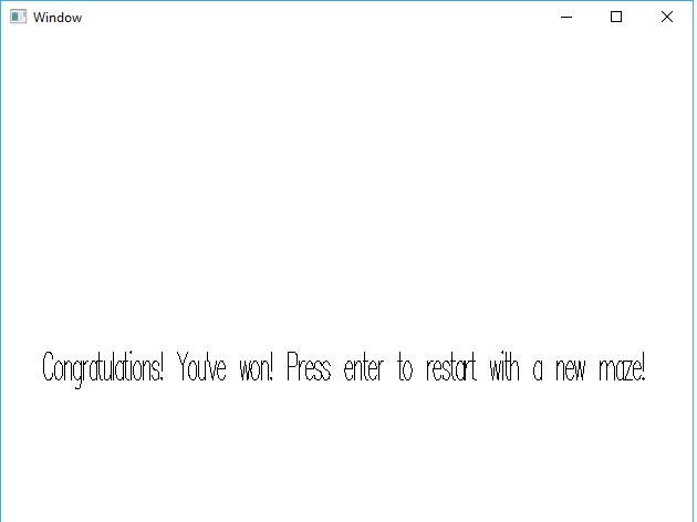
(Text "Congratulations! You've won!\
\Press enter to restart with a new maze!")
| otherwise = ...Note that Text here is the Gloss Picture constructor, not Data.Text. We also scale and translate it a bit to make the text appear on the screen. This is all we need to get the victory screen to appear on completion!
Restarting the Game
The last step is that we have to follow through on our process to restart the game if they hit enter! This involves changing our inputHandler to give us a brand new World. As with our other functions, we'll add a guard to handle the GameWon case:
inputHandler :: Event -> World -> World
inputHandler event w
  | worldResult w == GameWon = …
  | otherwise = case event of
    ...
We'll want to make a new case section that accounts for the user pressing the "Enter" key. All this section needs to do is call generateRandomMaze and re-initialize the world!
inputHandler event w
  | worldResult w == GameWon = case event of
      (EventKey (SpecialKey KeyEnter) Down _ _) ->
        let (newMaze, gen') = generateRandomMaze
              (worldRandomGenerator w) (25, 25)
        in  World (0, 0) (0, 0) (24, 24) newMaze GameInProgress gen'
      _ -> w
And with that, we're done! We can restart the game and navigate random mazes to our heart's content!
Conclusion
The ability to restart the game is great! But if we want to make our game re-playable instead of random, we'll need some way of storing mazes. In the next part, we'll look at some code for dumping a maze to an output format. We'll also need a way to re-load from this stored representation. This will ultimately allow us to make a true game with saving and loading state.
In preparation for that, you can read our series on Parsing. You'll especially want to acquaint yourself with the Megaparsec library. We go over this in Part 4 of the series!
Generating More Difficult Mazes!

In the last part of this series, we established the fundamental structures for our maze game. But our "maze" was still rather bland. It didn't have any interior walls, so getting to the goal point was trivial. In this next part, we'll look at an algorithm for random maze generation. This will let us create some more interesting challenges. In upcoming parts of this series, we'll explore several more related topics. We'll see how to serialize our maze definition. We'll refactor some of our data structures. And we'll also take a look at another random generation algorithm.
If you've never programmed in Haskell before, you should download our Beginners Checklist! It will help you learn the basics of the language so that the concepts in this series will make more sense. The State monad will also see a bit of action in this part. So if you're not comfortable with monads yet, you should read our series on them!
Getting Started
We represent a maze with the type Map.Map Location CellBoundaries. For a refresher, a Location is an Int tuple. And the CellBoundaries type determines what borders a particular cell in each direction:
type Location = (Int, Int)

data BoundaryType = Wall | WorldBoundary | AdjacentCell Location

data CellBoundaries = CellBoundaries
  { upBoundary :: BoundaryType
  , rightBoundary :: BoundaryType
  , downBoundary :: BoundaryType
  , leftBoundary :: BoundaryType
  }
An important note is that a Location refers to the position in discrete x,y space. That is, the first index is the column (starting from 0) and the second index is the row. Don't confuse row-major and column-major ordering! (I did this when implementing this solution the first time).
To generate our maze, we'll want two inputs. The first will be a random number generator. This will help randomize our algorithm so we can keep generating new, fresh mazes. The second will be the desired size of our grid.
import System.Random (StdGen, randomR)

…

generateRandomMaze
  :: StdGen
  -> (Int, Int)
  -> Map.Map Location CellBoundaries
generateRandomMaze gen (numRows, numColumns) = ...
A Simple Randomization Algorithm
This week, we're going to use a relatively simple algorithm for generating our maze. We'll start by assuming everything is a wall, and we've selected some starting position. We'll use the following depth-first-search pattern:
- Consider all cells around us
- If there are any we haven't visited yet, choose one of them as the next cell.
- "Break down" the wall between these cells, and put that new cell onto the top of our search stack, marking it as visited.
- If we have visited all other cells around us, pop this current location from the stack
- As long as there is another cell on the stack, choose it as the current location and continue searching from step 1.
There are several pieces of state we have to maintain throughout the process. So the State monad is an excellent candidate for this problem! Let's make a SearchState type for all these:
data SearchState = SearchState
  { randomGenerator :: StdGen
  , locationStack :: [Location]
  , currentBoundaries :: Map.Map Location CellBoundaries
  , visitedCells :: Set.Set Location
  }

dfsSearch :: State SearchState ()
dfsSearch = ...
Each time we make a random selection, we'll use the randomR function that returns the appropriate value as well as a new generator. Then we'll use a normal list for our search stack since we can push and pop from the top with ease. Next, we'll track the current state of the maze (it starts as all walls and we'll gradually break those down). Finally, there's the set of all cells we've already visited.
Starting Our Search!
To start our search process, we'll pull all our information out of the state monad, and examine the stack. If it's empty, we're done and can return! Otherwise, we'll want to consider the top location:
dfsSearch = do
  (SearchState gen locs bounds visited) <- get
  case locs of
    [] -> return ()
    (currentLoc : rest) -> do
      ...
Finding New Search Candidates
Given a particular location, we need to find the potential neighbors. We want to satisfy two conditions:
- It shouldn't be in our
visitedset. - The boundary to this location should be a
Wall
Then we'll want to use these properties to determine a list of candidates. Each candidate will contain 4 items:
- The next location
- The bounds we would use for the new location
- The previous location
- The new bounds for the previous location.
This seems like a lot, but it'll make more sense as we fill out our algorithm. With that in mind, here's the structure of our findCandidates function:
findCandidates
  :: Location -- Current location
  -> Map.Map Location CellBoundaries -- Current maze state
  -> Set.Set Location -- Visited Cells
  -> [(Location, CellBoundaries, Location, CellBoundaries)]
findCandidates currentLocation bounds visited = ...
Filling in this function consists of following the same process for each of the four directions from our starting point. First we check if the adjacent cell in that direction is valid. Then we create the candidate, containing the locations and their new boundaries. Since the location could be invalid, the result is a Maybe. Here's what we do for the "up" direction:
findCandidates =
  let currentLocBounds = fromJust $
        Map.lookup currentLocation bounds
      upLoc = (x, y + 1)
      maybeUpCandidate = case
        (upBoundary currentLocBounds, Set.member upLoc visited) of
        (Wall, False) -> Just
          ( upLoc
          , (fromJust $ Map.lookup upLoc bounds)
              { downBoundary = AdjacentCell currentLocation }
          , currentLocation
          , currentLocBounds { upBoundary = AdjacentCell upLoc }
          )
        ...
We replace the existing Wall elements with AdjacentCell elements in our maze map. This may seem like it's doing a lot of unnecessary work in calculating bounds that we'll never use. But remember that Haskell is lazy! Any candidate that isn't chosen by our random algorithm won't be fully evaluated. We repeat this process for each direction and then use catMaybes on them all:
findCandidates =
  let currentLocBounds = fromJust $ Map.lookup currentLocation bounds
      upLoc = (x, y + 1)
      maybeUpCandidate = …
      rightLoc = (x + 1, y)
      maybeRightCandidate = …
      downLoc = (x, y - 1)
      maybeDownCandidate = …
      leftLoc = (x - 1, y)
      maybeLeftCandidate = …
  in  catMaybes [maybeUpCandidate, maybeRightCandidate, … ]
Choosing A Candidate
Our search function is starting to come together now. Here's what we've got so far. If we don't have any candidates, we'll reset our search state by popping the current location off our stack. Then we can continue the search by making another call to dfsSearch.
dfsSearch = do
  (SearchState gen locs bounds visited) <- get
  case locs of
    [] -> return ()
    (currentLoc : rest) -> do
      let candidateLocs = findCandidates currentLoc bounds visited
      if null candidateLocs
        then put (SearchState gen rest bounds visited) >> dfsSearch
        else ...
But assuming we have a non-empty list of candidates, we'll need to choose one. This function will update most of our state elements, so we'll put in in the State monad as well:
chooseCandidate
  :: [(Location, CellBoundaries, Location, CellBoundaries)]
  -> State SearchState ()
chooseCandidate candidates = do
  (SearchState gen currentLocs boundsMap visited) <- get
  ...
First, we'll need to select a random index into this list, which assumes it is non-empty.:
chooseCandidate candidates = do
  (SearchState gen currentLocs boundsMap visited) <- get
  let (randomIndex, newGen) = randomR (0, (length candidates) - 1) gen
      (chosenLocation, newChosenBounds, prevLocation, newPrevBounds) =
        candidates !! randomIndex
Since we did the hard work of creating the new bounds objects up above, the rest is straightforward. We'll create our new state with different components.
We get a new random generator from the randomR call. Then we can push the new location onto our search stack. Next, we update the bounds map with the new locations. Last, we can add the new location to our visited array:
chooseCandidate candidates = do
  (SearchState gen currentLocs boundsMap visited) <- get
  let (randomIndex, newGen) = randomR (0, (length candidates) - 1) gen
      (chosenLocation, newChosenBounds, prevLocation, newPrevBounds) =
        candidates !! randomIndex
      newBounds = Map.insert prevLocation newPrevBounds
        (Map.insert chosenLocation newChosenBounds boundsMap)
      newVisited = Set.insert chosenLocation visited
      newSearchStack = chosenLocation : currentLocs
  put (SearchState newGen newSearchStack newBounds newVisited)
Then to wrap up our DFS, we'll call this function at the very end. Remember to make the recursive call to dfsSearch!
dfsSearch = do
  (SearchState gen locs bounds visited) <- get
  case locs of
    [] -> return ()
    (currentLoc : rest) -> do
      let candidateLocs = findCandidates currentLoc bounds visited
      if null candidateLocs
        then put (SearchState gen rest bounds visited) >> dfsSearch
        else (chooseCandidate candidateLocs) >> dfsSearch
Incorporating Our Search
As a last step in our process, we need to incorporate our search function. At the most basic level, we'll want to execute our DFS state function and extract the boundaries from it:
generateRandomMaze :: StdGen -> (Int, Int) -> Map.Map Location CellBoundaries
generateRandomMaze gen (numRows, numColumns) =
  currentBoundaries (execState dfsSearch initialState)
  where
    initialState :: SearchState
    initialState = ...
But we need to build our initial state. We'll start our search from a random location. Our initial stack and visited set will contain this location. Notice that with each random call, we use a new generator.
generateRandomMaze gen (numRows, numColumns) =
  currentBoundaries (execState dfsSearch initialState)
  where
    (startX, g1) = randomR (0, numColumns - 1) gen
    (startY, g2) = randomR (0, numRows - 1) g1

    initialState :: SearchState
    initialState = SearchState
      g2
      [(startX, startY)]
      … -- TODO Bounds
      (Set.fromList [(startX, startY)])
The last thing we need is our initial bounds set. For this, I'm going to tease the next part of the series. We'll write a function to parse a maze from a string representation (and reverse the process). Our encoding will represent a "surrounded" cell with the character 'F'. So we can represent a completely blocked maze like so:
generateRandomMaze gen (numRows, numCols) = …
  where
    …

    fullString :: Text
    fullString = pack . unlines $
      take numRows $ repeat (take numColumns (repeat 'F'))
Finally, we'll apply the mazeParser function in Megaparsec style. You'll have to wait a couple weeks to see how to implement that! It will give us the appropriate cell boundaries.
generateRandomMaze gen (numRows, numColumns) =
  currentBoundaries (execState dfsSearch initialState)
  where
    (startX, g1) = randomR (0, numColumns - 1) gen
    (startY, g2) = randomR (0, numRows - 1) g1

    initialState :: SearchState
    initialState = SearchState
      g2
      [(startX, startY)]
      initialBounds
      (Set.fromList [(startX, startY)])

    initialBounds :: Map.Map Location CellBoundaries
    initialBounds = case Megaparsec.runParser
      (mazeParser (numRows, numColumns) "" fullString of
        Right bounds -> bounds
        _ -> error "Couldn't parse maze for some reason!"

    fullString :: Text
    fullString = ...
You can also look at our Github repo for some details. You'll want the part-2 branch if you want more details about how everything works!
Conclusion
Generating random mazes is cool. But it would be nice if we could actually finish the maze we're running and do another one! Next week, we'll make some modifications to the game state so that when we finish with one maze, we'll have the option to try another random one!
If you're just getting started with Haskell, we have some great resources to get you going! Download our Beginners Checklist and read our Liftoff Series!
Building a Bigger World

Last week we looked at some of the basic components of the Gloss library. We made simple animations and simulations, as well as a very simple "game" taking player input. This week, we're going to start making a more complex game!
Our game will involve navigating a maze, from start to finish. In fact, this week, we're not even going to make it very "mazy". We're just going to set up an open grid to navigate around with our player. But over the course of these next few weeks, we'll add more and more features, like enemies and hazards. At some point, we'll have so many features that we'll need a more organized scheme to keep track of everything. At that point, we'll discuss game architecture. You can take a look at the code for this game on our Github repository. For this part, you'll want to look at the part-1 branch.
Game programming is only one of the many interesting ways we can use Haskell. Take a look at our Production Checklist for some more ideas!
Making Our World
As we explored in the last part, the World type is central to how we define our game. It is a parameter to all the important functions we'll write. Before we define our World though, let's define a couple helper types. These will clarify many of our other functions.
-- Defined in Graphics.Gloss
-- Refers to (x, y) within the drawable coordinate system
type Point = (Float, Float)

-- Refers to discrete (x, y) within our game grid.
type Location = (Int, Int)

data GameResult = InProgress | PlayerWin | PlayerLoss
Let's start our World type now with a few simple elements. We'll imagine the game board as a grid with a fixed size, with the tiles having coordinates like (0,0) in the bottom left. We'll want a start location and an ending location for the maze. We'll also want to track the player's current location as well as the current "result" of the game:
data  World = World
  { playerLocation :: Location
  , startLocation :: Location
  , endLocation :: Location
  , gameResult :: GameResult
  …
  }
Now we need to represent the "maze". In other words, we want to be able to track where the "walls" are in our grid. We'll make a data type to represent to boundaries for any particular cell. Then we'll stick a mapping from each location in our grid to its boundaries:
data BoundaryType = WorldBoundary | Wall | AdjacentCell Location

data CellBoundaries = CellBoundaries
  { upBoundary :: BoundaryType
  , rightBoundary :: BoundaryType
  , downBoundary :: BoundaryType
  , leftBoundary :: BoundaryType
  }

data  World = World
  { …
  , worldBoundaries :: Map Location CellBoundaries
  }
Populating Our World
Next week we'll look into how we can generate interesting mazes. But for now, our grid will only have "walls" on the outside, not in the middle. To start, we'll define a function that takes the number of rows and columns in our grid and a particular location. It will return the "boundaries" of the cell at that location. Each boundary tells us if there is a wall in one direction, or if we are clear to move to a different cell. All we need to check is if we're about to exceed the boundary in that direction.
simpleBoundaries :: (Int, Int) -> Location -> CellBoundaries
simpleBoundaries (numColumns, numRows) (x, y) = CellBoundaries
  (if y + 1 < numRows
    then AdjacentCell (x, y+1)
    else WorldBoundary)
  (if x + 1 < numColumns
    then AdjacentCell (x+1, y)
    else WorldBoundary)
  (if y > 0 then AdjacentCell (x, y-1) else WorldBoundary)
  (if x > 0 then AdjacentCell (x-1, y) else WorldBoundary)
Our main function now will loop through all the different cells in our grid and make a map out of them:
boundariesMap :: (Int, Int) -> Map.Map Location CellBoundaries
boundariesMap (numColumns, numRows) = Map.fromList
  (buildBounds <$> (range ((0,0), (numColumns, numRows))))
  where
    buildBounds :: Location -> (Location, CellBoundaries)
    buildBounds loc =
      (loc, simpleBoundaries (numColumns, numRows) loc)
Now we have all the tools we need to populate our initial world:
main = play
  windowDisplay
  white
  20
  (World (0, 0) (0,0) (24, 24) InProgress (boundariesMap (25, 25))
  drawingFunc ...
  inputHandler …
  updateFunc ...
Drawing Our World
Now we need to draw our world. We'll begin by passing a couple new parameters to our drawing function. We'll need offset values that will tell us the Point in our geometric coordinate system for the Location (0,0). We'll also take a floating point value for the cell size. Then we will also, of course, take the World as a parameter:
drawingFunc :: (Float, Float) -> Float -> World -> Picture
drawingFunc (xOffset, yOffset) cellSize world = …
Before we do anything else, let's define a type called CellCoordinates. This will contain the Points for the center and four corners of a cell in our grid.
data CellCoordinates = CellCoordinates
  { cellCenter :: Point
  , cellTopLeft :: Point
  , cellTopRight :: Point
  , cellBottomLeft :: Point
  , cellBottomRight :: Point
  }
Next, let's define a conversion function from a Location to one of the coordinate objects. This will take the offsets, cell size, and the desired location.
locationToCoords ::
  (Float, Float) -> Float -> Location -> CellCoordinates
locationToCoords (xOffset, yOffset) cellSize (x, y) = CellCoordinates
  (centerX, centerY) -- Center
  (centerX - halfCell, centerY + halfCell) -- Top Left
  (centerX + halfCell, centerY + halfCell) -- Top Right
  (centerX - halfCell, centerY - halfCell) -- Bottom Left
  (centerX + halfCell, centerY - halfCell) -- Bottom Right
  where
    (centerX, centerY) =
      ( xOffset + (fromIntegral x) * cellSize
      , yOffset + (fromIntegral y) * cellSize)
    halfCell = cellSize / 2.0
Now we can go ahead and make the first few simple pictures in our game. We'll have colored polygons for the start and end locations, and a circle for the player token. The player marker is easiest:
drawingFunc (xOffset, yOffset) cellSize world =
  Pictures [startPic, endPic, playerMarker]
  where
    conversion = locationToCoords (xOffset, yOffset) cellSize
    (px, py) = cellCenter (conversion (playerLocation world))
    playerMarker = translate px py (Circle 10)
    startPic = …
    endPic = ...
We find its coordinates through our conversion, and then translate a circle. For our start and end points, we'll want to do something similar, except we want the corners, not the center. We'll use the corners as the points in our polygons and draw these polygons in appropriate colors.
drawingFunc (xOffset, yOffset) cellSize world =
  Pictures [startPic, endPic, playerMarker]
  where
    conversion = locationToCoords (xOffset, yOffset) cellSize
    ...
    startCoords = conversion (startLocation world)
    endCoords = conversion (endLocation world)
    startPic = Color blue (Polygon
      [ cellTopLeft startCoords
      , cellTopRight startCoords
      , cellBottomRight startCoords
      , cellBottomLeft startCoords
      ])
    endPic = Color green (Polygon
      [ cellTopLeft endCoords
      , cellTopRight endCoords
      , cellBottomRight endCoords
      , cellBottomLeft endCoords
      ])
Now we need to draw the wall lines. So we'll have to loop through the wall grid, drawing the relevant lines for each individual cell.
drawingFunc (xOffset, yOffset) cellSize world = Pictures
  [mapGrid, startPic, endPic, playerMarker]
  where
  …
    mapGrid = Pictures $concatMap makeWallPictures
      (Map.toList (worldBoundaries world))

    makeWallPictures :: (Location, CellBoundaries) -> [Picture]
    makeWallPictures ((x, y), CellBoundaries up right down left) = ...
When drawing the lines for an individual cell, we'll use thin lines when there is no wall. We can make these with the Line constructor and the two corner points. But we want a separate color and thickness to distinguish an impassable wall. In this second case, we'll want two extra points that are offset so we can draw a polygon. Here's a helper function we can use:
drawingFunc (xOffset, yOffset) cellSize world = ...
  where
   ...
    drawEdge :: (Point, Point, Point, Point) ->
                 BoundaryType -> Picture
    drawEdge (p1, p2, _, _) (AdjacentCell _) = Line [p1, p2]
    drawEdge (p1, p2, p3, p4) _ =
      Color blue (Polygon [p1, p2, p3, p4])
Now to apply this function, we'll need to do a little math to dig out all the individual coordinates out of this cell.
drawingFunc (xOffset, yOffset) cellSize world =
  Pictures [mapGrid, startPic, endPic, playerMarker]
  where
    ...
    makeWallPictures :: (Location, CellBoundaries) -> [Picture]
    makeWallPictures ((x,y), CellBoundaries up right down left) =
      let coords = conversion (x,y)
          tl@(tlx, tly) = cellTopLeft coords
          tr@(trx, try) = cellTopRight coords
          bl@(blx, bly) = cellBottomLeft coords
          br@(brx, bry) = cellBottomRight coords
      in  [ drawEdge (tr, tl, (tlx, tly - 2), (trx, try - 2)) up
          , drawEdge (br, tr, (trx-2, try), (brx-2, bry)) right
          , drawEdge (bl, br, (brx, bry+2), (blx, bly+2)) down
          , drawEdge (tl, bl, (blx+2, bly), (tlx+2, tly)) left
          ]
But that's all we need! Now our drawing function is complete!
Player Input
The last thing we need is our input function. This is going to look a lot like it did last week. We'll only be looking at the arrow keys. And we'll be updating the player's coordinates if the move they entered is valid. To start, let's figure out how we get the bounds for the player's current cell (we'll assume the location is in our map).
inputHandler :: Event -> World -> World
inputHandler event w = case event of
  (EventKey (SpecialKey KeyUp) Down _ _) -> ...
  (EventKey (SpecialKey KeyDown) Down _ _) -> ...
  (EventKey (SpecialKey KeyRight) Down _ _) -> ...
  (EventKey (SpecialKey KeyLeft) Down _ _) -> ...
  _ -> w
  where
    cellBounds = fromJust $ Map.lookup (playerLocation w) (worldBoundaries w)
Now we'll define a function that will take an access function to the CellBoundaries. It will determine what our "next" location is.
inputHandler :: Event -> World -> World
inputHandler event w = case event of
  ...
  where
    nextLocation :: (CellBoundaries -> BoundaryType) -> Location
    nextLocation boundaryFunc = case boundaryFunc cellBounds of
      (AdjacentCell cell) -> cell
      _ -> playerLocation w
Finally, we pass the proper access function for the bounds with each direction, and we're done!
inputHandler :: Event -> World -> World
inputHandler event w = case event of
  (EventKey (SpecialKey KeyUp) Down _ _) ->
    w { playerLocation = nextLocation upBoundary }
  (EventKey (SpecialKey KeyDown) Down _ _) ->
    w { playerLocation = nextLocation downBoundary }
  (EventKey (SpecialKey KeyRight) Down _ _) ->
    w { playerLocation = nextLocation rightBoundary }
  (EventKey (SpecialKey KeyLeft) Down _ _) ->
    w { playerLocation = nextLocation leftBoundary }
  _ -> w
  where
    ...
Tidying Up
Now we can put everything together in our main function with a little bit of glue.
main :: IO ()
main = play
  windowDisplay
  white
  20
  (World (0, 0) (0,0) (24,24) (boundariesMap (25, 25)))
  (drawingFunc (globalXOffset, globalYOffset) globalCellSize)
  inputHandler
  updateFunc

updateFunc :: Float -> World -> World
updateFunc _ = id
Note that for now, we don't have much of an "update" function. Our world doesn't change over time. Yet! We'll see in the coming weeks what other features we can add that will make use of this.
Conclusion
So we've finished stage 1 of our simple game! You can explore the part-1 branch on our Github repository to look at the code if you want! Come back next week and we'll explore how we can actually create a true maze, instead of an open grid. This will involve some interesting algorithmic challenges!
For some more ideas of advanced Haskell libraries, check out our Production Checklist. You can also read our Web Skills Series for a more in-depth tutorial on some of those ideas.
Making a Glossy Game! (Part 1)

I've always had a little bit of an urge to try out game development. It wasn't something I associated with Haskell in the past. But recently, I started learning a bit about game architecural patterns. I stumbled on some ideas that seemed "Haskell-esque". I learned about the Entity-Component-System model, which suits typeclasses rather than object-oriented design.
So I've decided to do a few articles on writing a basic game in Haskell. We'll delve more into these architectural ideas later in the series. But to start, we have to learn a few building blocks! The first couple weeks will focus on the basics of the Gloss library. This library has some simple tools for creating 2D graphics that we can use to make a game. Frequent readers of this blog will note a lot of commonalities between Gloss and the Codeworld library we studied a while back. In this first part, we'll learn some basic combinators.
If you're looking for some more practical usages of Haskell, we have some tools for you! Download our Production Checklist to learn many interesting libraries you can use! You can also read our Haskell Web Skills series to go a bit more in depth!
A Basic Gloss Tutorial
The get started with the Gloss library, let's draw a simple picture using the display function. All this does is make a full screen window with a circle in the middle.
-- Always imported
import Graphics.Glass

main :: IO ()
main = display FullScreen white (Circle 80)
All the arguments here are pretty straightforward. The program opens a full screen window and displays a circle against a white background. We can make the window smaller by using InWindow instead of FullScreen for the Display type. This takes a window "name", as well as dimensions for the size and offset of the window.
windowDisplay :: Display
windowDisplay = InWindow "Window" (200, 200) (10, 10)

main :: IO ()
main = display windowDisplay white (Circle 80)
The primary argument here is this last one, a Picture using the Circle constructor. We can draw many different things, including circles, lines, boxes, text, and so on. The Picture type also allows for translation, rotation, and aggregation of other pictures.
Animating
We can take our drawing to the next level by using the animate function. Instead of only drawing a static picture, we'll take the animation time as an input to a function. Here's how we can provide an animation of a growing circle:
main = animate windowDisplay white animationFunc

animationFunc :: Float -> Picture
animationFunc time = Circle (2 * time)
Simulating
The next stage of our program's development is to add a model. This allows us to add state to our animation so that it is no longer merely a function of the time. For our next example, we'll make a pendulum. We'll keep two pieces of information in our model. These are the current angle ("theta") and the derivative of that angle ("dtheta"). The simulate function takes more arguments than animate. Here's the skeleton of how we use it. We'll go over the new arguments one-by-one.
type Model = (Float, Float)

main = simulate
  displayWindow
  white
  simulationRate
  initialModel
  drawingFunc
  updateFunc
  where
    simulationRate :: Int
    simulationRate = 20

    initialModel :: Model
    initialModel = (0,0)

    drawingFunc :: Model -> Picture
    drawingFunc (theta, dtheta) = …

    updateFunc :: ViewPort -> Float -> Model -> Model
    updateFunc _ dt (theta, dtheta) = ...
The first extra argument (simulationRate) tells us how many model steps per second. Then we have our initial model. Then there's a function taking the model and telling us how to draw the picture. We'll fill this in to draw a line at the appropriate angle.
drawingFunc :: Model -> Picture
drawingFunc (theta, dtheta) = Line [(0, 0), (50 * cos theta, 50 * sin theta)]
Finally, we have an updating function. This takes the view-port, which we won't use. It also takes the amount of time for this simulation step (dt). Then it takes a current model. It uses these to determine the new model. We can fill this in with a little bit of trigonometry. Then we'll have a working pendulum simulation!
updateFunc :: ViewPort -> Float -> Model -> Model
updateFunc _ dt (theta, dtheta) = (theta + dt * dtheta, dtheta - dt * (cos theta))
Playing a Game
The final element we need to make a playable game is to accept user input. The play function provides us what we need here. It looks like the simulate function except for an extra function for handling input. We're going to make a game where the user can move a circle around with the arrow keys. We'll add an extra mechanic where the circle keeps trying to move back towards the center. Here's the skeleton:
type World = (Float, Float)

main :: IO ()
main = play
  windowDisplay
  white
  20
  (0, 0)
  drawingFunc
  inputHandler
  updateFunc

drawingFunc :: World -> Picture
drawingFunc (x, y) = ...

inputHandler :: Event -> World -> World
inputHandler event (x, y) = ...

updateFunc :: Float -> World -> World
updateFunc dt (x, y) = ...
Our World will represent the current location of our circle. The drawing function will draw a simple circle, translated by this amount.
drawingFunc :: World -> Picture
drawingFunc (x, y) = translate x y (Circle 20)
Now for our input handler, we only care about a few inputs. We'll read the up/down/left/right arrows, and adjust the coordinates:
inputHandler :: Event -> World -> World
inputHandler (EventKey (SpecialKey KeyUp) Down _ _) (x, y) = (x, y + 10)
inputHandler (EventKey (SpecialKey KeyDown) Down _ _) (x, y) = (x, y - 10)
inputHandler (EventKey (SpecialKey KeyRight) Down _ _) (x, y) = (x + 10, y)
inputHandler (EventKey (SpecialKey KeyLeft) Down _ _) (x, y) = (x - 10, y)
inputHandler _ w = w
Finally, let's write our "update" function. This will keep trying to move the circle's coordinates towards the center of the frame:
updateFunc :: Float -> World -> World
updateFunc _ (x, y) = (towardCenter x, towardCenter y)
  where
    towardCenter :: Float -> Float
    towardCenter c = if abs c < 0.25
      then 0
      else if c > 0
        then c - 0.25
        else c + 0.25
And that's it, we have our miniature game!
Conclusion
Hopefully this article gave you a good, quick overview on the basics of the Gloss library. Next week, we'll start making a more complicated game with a more interesting model!
We have other resources for the more adventurous Haskellers out there! Download our Production Checklist and read our Haskell Web Skills Series!
Extending Haskell's Syntax!

When you're starting out with Haskell, compiler extensions seem a little weird. And in a way, they are. It's strange to think that you need to "opt in" to certain compiler features. And as a beginner, it can be overwhelming to think you need to know the meaning of certain odd terms. I still remember how some of the first Haskell code I worked on had at least 10 extensions in every file. And I didn't have a clue what they meant!
But there are good reasons for certain features to be "opt in". They might make the compilation process longer. Or they might make some types of code less performant. But there are many extensions you can use that can make you life easier without worrying. And many extensions are easy to learn, so you can get the hang of the concept.
In this article, we’re going to do a quick run-down of some simple extensions. You’ve probably heard of at least of few of these. But it’s always good to keep learning. None of these are too advanced. For the most part, they allow you to use some more syntactic sugar and write cleaner code. So they’re pretty uncontroversial and you should feel free to use them in any file you want. Learning a few of these will help you get more comfortable so you can tackle harder extensions when you need to.
For some more tools to take your Haskell to the next level, download our Production Checklist! You can also read our Haskell Web Series for some tutorials.
Overloaded Strings
We’ve done one article already on overloaded strings. But here’s another quick summary. There are five different string types in Haskell. By default, Haskell assumes that whenever you use a string literal, you intend for it to be the String type.
-- Defaults as String
aString = "Hello"

-- The following will NOT WORK (by default)
aText :: Text
aText = "Hello"
This is annoying, because String is generally inferior to the other string types. You should be using Text most of the time for performance reasons. If we use the OverloadedStrings extension, then we can use literals for any of these string types!
{-# LANGUAGE OverloadedStrings #-}

-- Now this works!
aText :: Text
aText = "Hello"

aByteString :: ByteString
aByteString = "Hello"
And, in fact, you can use string literals for any type you want! All you have to do is create an instance of the IsString class for it by defining the fromString function.
newtype Name = Name String

instance IsString Name where
  fromString s = Name s

myName :: Name
myName = "James"
This is one of the most common and simplest extensions you can use, so it's a great one to start with!
Lambda Case
Lambda case is another simple extension, but it isn’t quite as common as overloaded strings. It helps clean up a particular syntax wart that comes up from time to time. Consider a function where we take a single argument, and then immediately run a case statement on it:
useParseResult :: Either ParseError Result -> IO ()
useParseResult x = case x of
  Left parseError -> …
  Right goodResult -> ...
You could do a direct pattern match, but sometimes this is impossible if you’re in-lining the function. Notice that we use a one-letter variable name x. We could come up with a better name. But it seems like a waste since we don't use this variable anywhere else in the function definition. If would be nice if we could remove it altogether.
The LambdaCase extension allows this by providing the following syntactic sugar. You can use case as if it were the argument of a lambda expression, and then immediately do the pattern match:
{-# LANGUAGE LambdaCase #-}

useParserResult :: EitherParseError Result -> IO ()
useParserResult = \case ->
  Left parseError -> ...
  Right goodResult -> ...
At the end of the day, it’s a small difference. But it's a nice little trick you can use to save yourself some unneeded variable names.
Bang Patterns
Haskell is lazy by default. But there are certain situations where you need a strict value as an input to your function. This means the value should get evaluated BEFORE the function gets run. This is a little tricky to do with normal Haskell syntax. Consider this function:
bangTest :: Bool -> Int -> Int
bangTest b i = if b then 42 else 2 * i
If the boolean is true, laziness means we never evaluate the int argument. Hence the following works:
>> bangTest True undefined
42
But if we want that situation to fail, we need to use seq:
bangTest b i = seq i $ if b then 42 else 2 * i

…
>> bangTest True undefined
***Exception: Prelude.undefined
The BangPatterns extension allows us to use the bang character ! to specify that the function should be strict in an argument. So instead of using seq like above, we can get the same behavior like so:
bangTest :: Bool -> Int -> Int
bangTest b !i = if b then 42 else 2 * i

…

>> bangTest True undefined
***Exception: Prelude.undefined
Even without this extension, you can use strictness annotations in type definitions. Consider this example:
data Person = Person String

printName :: Bool -> Person -> IO ()
printName b (Person name) = if b
  then putStrLn "Hello"
  else putStrLn name

…
>> printName True (Person undefined)
Hello
But we can also make person strict in its string argument like so:
data Person = Person !String

…

>> printName True (Person undefined)
*** Exception: Prelude.undefined
And again, this last example works even without the extension!
Type Operators
Haskell is sometimes criticized for an abundance of confusing operators. This next syntax extension does not ease this criticism! But it does provide some neat new possibilities when defining types! Here's an example with the Servant library. It requires both DataKinds and TypeOperators, but we'll focus on the latter.
{-# LANGUAGE DataKinds #-}
{-# LANGUAGE TypeOperators #-}

type PersonAPI =
       "person" :> Capture "personid" Int :> Get '[JSON] Person
  :<|> "person" :> ReqBody '[JSON] Person :> Post '[JSON] Int
As a reminder, we've defined a type up there, not a normal expression! This means the :> and :<|> operators are actually constructors! Let's define an example for ourselves. Suppose we have a simple type that wraps a couple other types in a pair:
data MyPair a b = MyPair a b

collection :: MyPair [Int] [String]
...
Now suppose we want to join more types together. We can do this by nesting MyPair instances, but the type signatures will get messy:
bigCollection :: MyPair [Int] (MyPair [String] (Map String Int))But we can define a type operator that allows us to join these together!
infixr 8 +>>
type (t1 +>> t2) = MyPair t1 t2
And now we can get far cleaner signatures!
collection :: [Int] +>> [String]

bigCollection :: [Int] +>> [String] +>> Map String Int
Haskell lets us make complex recursive structures with many different type parameters. Type operators help us keep the signatures concise when we do this!
Tuple Sections
We've got one last trick for you. The TupleSections extension makes tuples easier to work with. Even without an extension can use the comma operator to build tuples like so:
combined :: (Int, String)
combined = (,) 5 "Hello"

combined3 :: (Int, String, Float)
combined3 = (,,) 5 "Hello" 2.3
But suppose we want to apply a function where we hardcode a particular value of a tuple. We'd need a separate definition of this function:
injectHello :: Int -> Float -> (Int, String, Float)
injectHello i f = (i, "Hello", f)

fetchInt :: IO Int

fetchFloat :: IO Float

combined :: IO (Int, String, Float)
combined = injectHello <$> fetchInt <*> fetchFloat
But with TupleSections, we can create a constructor that already has "Hello" built in! We can then apply it as a function with using another definition!
{-# LANGUAGE TupleSections #-}

combined :: IO (Int, String, Float)
combined = (,"Hello",) <$> fetchInt <*> fetchFloat
This is another useful little trick that let's us skip annoying in-between definitions. When you add up all these small things, it can go a long way towards cleaner code!
Conclusion
The ecosystem of Haskell compiler extensions is very large. As a beginner, it can be hard to know where to start. But many extensions are simple. In this article, we went over a couple simple ones and a couple more complicated ones. Once you get familiar with one or two, the concept starts making a lot more sense.
For some more ideas on taking your Haskell to the next level, check out our Production Checklist! It has a list of libraries for cool purposes like writing servers and using databases!
Modifying a Library!

Sometime last year, I wrote an article about advanced Stack techniques. We discussed one hypothetical case where a library had a bug. The solution here was to fork the repository and use a Github location in stack.yaml.
I recently came across an easy example of doing this and thought I'd share it. We can see how to incorporate the change without stressing about its complexity. Even if you're only a beginner, this is a good skill to learn now!
You'll need some background on Stack first though! If you've never used Stack before, take a look at our Stack mini-course to learn more!
Background
I've been doing a bit of work lately with the persistent-migration library. This library lets us set up manual migrations for a Persistent schema we've set up through template Haskell. See this article for more on that topic.
The migrations library has a couple functions that let us run some SQL operations. They live in the SqlPersistT monad, as we would expect. However, something's a little off about them:
getMigration ::
  MigrateSettings -> Migration -> SqlPersistT IO [MigrateSql]

runMigration ::
  MigrateSettings -> Migration -> SqlPersistT IO ()
We can see that these functions restrict us to using SqlPersistT on top of the normal IO monad. But in most cases with Persistent, I use the withPostgresqlConn function. This adds a MonadLogger constraint. Thus IO doesn't cut it. Most functions have a type signature looking like this:
databaseOp :: SqlPersistT (LoggingT IO) aSo we can't interoperate as easily as we'd like between our normal database operations, and these migration functions. The solution is that the migration functions should be more general in what monads they can use. This will be an easy fix, as we'll see. But first, we have to find a way to get our own version of the code.
Getting Started
The persistent-migration library is on Github here. So we can make a fork of the repository, and clone that to our machine:
git clone https://github.com/jhb563/peristent-migrationNow we'll follow the build instructions in the Developing.md file to get set up. Some of the tests fail on my machine, but we'll ignore that for this article.
Making Our Code Fixes
The code fixes turn out to be very easy. We can go into the relevant module and change the type signatures so they are more general:
module Database.Persistent.Migration.Postgres where

...

getMigration :: (MonadIO m) =>
  MigrateSettings -> Migration -> SqlPersistT m [MigrateSql]

runMigration :: (MonadIO m) =>
  MigrateSettings -> Migration -> SqlPersistT m ()
Even in the worst case, the only changes we would need to make here would be to add liftIO calls in various places. But it turns out that this change doesn't break anything! The library still builds, and all the tests that were passing before still pass.
So now we can commit this change to our fork and push it to the repository.
Incorporating the Fix
Now we have to use our own fork as an alternative to the version of the library on Hackage. Before, the extra-deps section in ourstack.yaml` looked like this:
extra-deps:
  - persistent-migration-0.1.0
This indicates we would grab the code from Hackage. But now we can use an alternative package format to reference our Github repository. Here's what we change it to:
extra-deps:
  - git: https://github.com/jhb563/persistent-migration.git
    commit: 9f9c5035efe
And now we've got our own fork as a dependency for our project! We can write code like so:
doMigrations :: SqlPersistT (LoggingT IO) a
doMigrations = do
  runMigration defaultSettings migration
  ...
And everything works! Our code builds!
Potential Issues
Now, an approach like this can lead to some possible issues. We're now disconnected from the original repository. So if there was a new release, we'd have to do a bit more work to pull those changes into our own repository. Still, this isn't too difficult. One solution to this is to submit a pull request with our changes. If it gets accepted, they'll be in the next release! Then we can go back to using the version on Hackage!
Conclusion
In this article, we did a quick overview of how to make our own changes to libraries. We cloned the repository, made a code change, and added our fork as a dependency. Obviously, most of the changes you'll want to make aren't as simple as this one was. But it's good to use an example where all we're doing is tackling the issue of getting the code into our code base!
For a broad overview of how to use the Stack program, make sure to check out of Stack Mini-course! If you've never written any Haskell before, you can also look at our Beginners Checklist!
Shareable Haskell with Jupyter!
In the last couple weeks, we've discussed a couple options for Haskell IDEs, like Atom and IntelliJ. But there's another option I'll talk about this week. Both our IDE setups are still most useful for fully-fledged projects. But if you're writing some quick and dirty one-off code, they can be a little cumbersome to work with.
This other option is Jupyter with IHaskell. It's like IPython, for those who have used that. I got the idea when the good folks at Tweag made a blog post with it. Jupyter was originally intended for making quick Python data science scripts. It allows a nice UI for making data visualizations. Thanks to the hard work of Andrew Gibiansky, there is a Haskell kernel for Jupyter! In this article, we'll discuss some quick approaches to using it.
IHaskell is actually a great tool when you're first learning Haskell! If you've never programmed in Haskell before, you can read our Liftoff Series and follow along with the code examples! You can write them using IHaskell instead of making a Stack project!
Installing
If you want to make a full-fledged Jupyter notebook, you'll need to install Jupyter first. The most heavy-duty but easiest way would be to use the Anaconda distribution. But there are also other options like pip.
After that, you'll need to install the Haskell kernel for it. Unfortunately, you can't do this on a Windows machine. You either need a Mac, Linux or a virtual box. The instructions for these systems are well documented in the README. In short, you need to sort out your Python dependencies, grab the Github repo, and build the project.
Now if you're on Windows, or you don't want to install the full Jupyter system, you can try out IHaskell online. Head to this Binder page, make a new notebook, and get cracking!
Making a Basic Example
In our notebook, we can write Haskell code as if we're in a file, but evaluate it as if we're in GHCI. A quick look at the .cabal file will reveal the libraries we have easy access to in this notebook setup. We can see for instance that we have stalwarts such as mtl, aeson, and split. Using this last library, we can write the following snippet:

Then we press shift+enter to finish the cell and it gets evaluated. Evaluations work as in GHCI. Anything you assign to a variable name will be usable later on in your notebook. Then the final expression you put will get printed. So we'll see output like so:

Then we can use the items we named in another snippet like this:

Since we also have access to the Aeson library, we can serialize our list like so:

As a final note it is easy to create multiline definitions and use those! This is a big improvement over GHCI. It would be very annoying to define a new data type, for instance:

Exporting the Notebook
Now one of the awesome things about Jupyter notebooks is that it's easy to share your work! There's an option off the file menu for downloading your notebooks. There are a great many options, including Haskell source files, pdfs, and HTML documents. These last two can be extremely useful if you want to make a presentation!

Conclusion
As I move forward with MMH, I'm definitely going to explore using notebooks like this more. It should provide a better reader experience than what I have now. I'll also be looking at migrating some of our existing permanent content to Jupyter. The lack of Windows functionality for Haskell is unfortunate, but I'll find a way around it.
Jupyter IHaskell is a great way to get familiar with the basics of Haskell without downloading any of the tools. But at some point, you'll need these! Read our Liftoff Series and download our Beginners Checklist to find out more!
Another IDEa: Haskell and IntelliJ!

Last week we explored one way to get a nice development environment for Haskell. We used the Atom text editor, which has a couple Haskell plugins and is quite hackable.
But there's another option I hadn't considered at all during that article. This is the IntelliJ IDE. It's primary use is Java and Android development. But like Atom, Visual Studio, and other IDEs, it has a rich library of plugins. And one of these is a Haskell environment!
This week, we'll see how to configure IntelliJ to work with Haskell. We'll see how we can get a nifty Haskell environment set up with the same features we had in Atom. I'm working on a Windows machine, but you should be able to do all these steps on a Mac as well.
An IDE is no substitute for basic knowledge though! If you're new to Haskell, getting a good dev setup will help. But you should also read our Liftoff Series and download our Beginners Checklist! These will give you some other tools you'll need!
Installation and Setup
Getting started with IntelliJ is quite easy. Installing the editor works through the normal wizard. You'll have a lot of options for different plugins to install immediately. A lot of these are Java specific so you won't need them. But once you've done that you can also install the IntelliJ-Haskell plugin. In my case, I also installed a Vim plugin for those keybindings.
There's a little bit of trickiness involved in setting your project up to build with Stack. When you first install the plugin, it will ask you what program to use to "build" a project. This means you'll need to locate your stack executable in the file finder so you can drag it in. On Windows this will mean showing hidden folders in the finder. You might also need to use the where command in the terminal to help (instead of which from Linux). Once you've done this though, you should be good!
Keyboard Shortcuts
When working with Atom, we stressed the importance of keyboard shortcuts. These can streamline our workflow a lot. IntelliJ also allows a good deal of customization options for these. The main thing to know is that you need to hit ctrl+alt+s to get to the settings menu. Then you can find the keymap on the side panel. From here you can customize pretty much anything. The big ones for me were building the project and manipulating panels.
The ability to search for commands is very useful. I found it a lot easier to alter commands for, say, splitting windows then I did in Atom. My current setup involves the following combinations:
Build Project: Ctrl+Alt+Shift+B
Split Screen Vertically: Ctrl+Alt+Shift+Right
Split Screen Horizontally: Ctrl+Alt+Shift+Down
Next/Previous Split: Ctrl+Shift+[Right/Left]
Unsplit: Ctrl+Alt+Shift+U
Toggle Bottom Terminal: Ctrl+Shift+Up
For what it's worth, I'll also note that the Vim keybindings are better than I had in Atom. Moving around with lines and saving files with :w work, for a couple examples.
Haskell Features
This is where the IntelliJ plugin shines. Lots of features work right out of the box. For instance, it knows to using hlint and highlights any code with lints. Compilation hints show up automatically. There's even a good deal of auto-completion from libraries for expressions and types. Integration with Hoogle is fairly straightforward.
Best of all, it seems to me that these features work across projects with different GHC versions. As far as I can tell you don't need to manually install ghc-mod and worry about it's version, as you did with Atom. Given the difficulties I had setting up Atom to work with these features, this was a major relief.
Git Integrations
We didn't go over version control last week. But it's another vital component in any developer's workflow, so IDE integration is a big plus. Both Atom and IntelliJ have good support for Github, which is excellent news! Both come with batteries included when it comes to all the common Git operations we want. You can make new branches, add commits, push and pull with ease. Both allow you to bind these to keys, allowing you the freedom to streamline your workflow even more.
Disadvantages
If I were to find one fault with my IntelliJ setup, it's that project setup can involve a lot of loading time. When you add a new library to the .cabal file, you need to run the Tools->Haskell->Update Settings command. The IDE will take a little while to reset everything to account for this. Having said that, a lot of that loading time goes into getting all the appropriate libraries to set up. This enables all the nice features I mentioned earlier. So I suppose that's the price you pay. Atom is also sometimes slow, for its part. But the program itself isn't quite as bulky as IntelliJ, which has a lot of extra features you probably won't need.
One last note is that IntelliJ will add a .idea folder to your project directory. Make sure to add this to your .gitignore!
Conclusion
All in all working with IntelliJ/HaskelIDE has been a good experience so far. It has all the features I'm looking for, and setup is a bit easier than Atom. Long loads can hold me back at times, but it's usually fine. Again, you can take a look at the Github page for the project for some more details. I highly recommend trying out this plugin! Much love to Rik van der Kleij, the author!
A full IDE setup will really help you get started learning Haskell! But you also need some other tools and knowledge. Download our Beginners Checklist for some other tools you'll need. Also take a look at our Stack mini-course to learn more about setting up a Haskell project!
Upgrading My Development Setup!

In the last year or so, I haven't actually written as much Haskell as I'd like to. There are a few reasons for this. First, I switched to a non-Haskell job, meaning I was now using my Windows laptop for all my Haskell coding. Even on my previous work laptop (a Mac), things weren't easy. Haskell doesn't have a real IDE, like IntelliJ for Java or XCode for iOS development.
Besides not having an IDE, Windows presents extra pains compared to the more developer-friendly Mac. And it finally dawned on me. If I, as an experienced developer, was having this much friction, it must be a nightmare for beginners. Many people must be trying to both learn the language AND fight against their dev setup. So I decided to take some time to improve how I program so that it'll be easier for me to actually do it.
I wanted good general functionality, but also some Haskell-specific functions. I did a decent amount of research and settled on Atom as my editor of choice. In this article, we'll explore the basics of setting up Atom, what it offers, and the Haskell tools we can use within it. If you're just starting out with Haskell, I hope you can take these tips to make your Haskell Journey easier.
Note that many tips in this article won't work without the Haskell platform! To start with Haskell, download our Beginners Checklist, or read our Liftoff Series!
Goals
It's always good to begin with the end in mind. So before we start out, let's establish some goals for our development environment. A lot of these are basic items we should have regardless of what language we're using.
- Autocomplete. Must have for terms within the file. Nice to have for extra library functions and types.
- Syntax highlighting.
- Should be able to display at least two code files side-by-side, should also be able to open extra files in tabs.
- Basic file actions should only need the keyboard. These include opening new files to new tabs or splitting the window and opening a new file in the pane.
- Should be able to build code using the keyboard only. Should be able to examine terminal output and code at the same time.
- Should be able to format code automatically (using, for instance, Hindent)
- Some amount of help filling in library functions and basic types. Should be able to coordinate types from other files.
- Partial compilation. If I make an obvious mistake, the IDE should let me know immediately.
- Vim keybindings (depends on your preference of course)
With these goals in mind, let's go ahead and see how Atom can help us.
Basics of Atom
Luckily, the installation process for Atom is pretty painless. Using the Windows installer comes off without a hitch for me. Out of the box, Atom fulfills most of the basic requirements we'd have for an IDE. In fact, we get all our 1-4 goals without putting in any effort. The trick is that we have to learn a few keybindings. The following are what you'll need to open files.
- Ctrl+P - Open a new tab with a file using fuzzy find
- Ctrl+K + Direction (left/right/up/down arrow) - Open a new pane (will initially have the same file as before).
- Ctrl+K + Ctrl+Direction - Switch pane focus
Those commands solve requirements 3 and 4 from our goals list.
Another awesome thing about Atom is the extensive network of easy-to-install plugins. We'll look at some Haskell specific items below. But to start, we can use the package manager to install vim-mode-improved. This allows most Vim keybindings, fulfilling requirement 9 from above. There are a few things to re-learn with different keystrokes, but it works all right.
Adding Our Own Keybindings
Since Atom is so Hackable, you can also add your own keybindings and change ones you don't like. We'll do one simple example here, but you can also check out the documentation for some more ideas. One thing we'll need for goal #5 is to make it easier to bring up the bottom panel within atom. This is where terminal output goes when we run a command. You'll first want to open up keymap.cson, which you can do by going to the file menu and click Keymap….
Then you can add the following lines at the bottom:
'atom-workspace':
  'ctrl-shift-down': 'window:toggle-bottom-dock'
  'ctrl-shift-up': 'window:toggle-bottom-dock'
First, we scope the command to the entire atom workspace. (We'll see an example below of a command with a more limited scope). Then we assign the Ctrl+Shift+Down Arrow key combination to toggle the bottom dock. Since it's a toggle command, we could repeat the command to move it both up and down. But this isn't very intuitive, so we add the second line so that we can also use the up arrow to bring it up.
A super helpful tool is the key binding resolver. At any point, you can use ctrl+. (control key plus the period key) to bring up the resolver. Then pressing any key combination will bring up the commands Atom will run for it. It will highlight the one it will pick in case of conflicts. This is great for finding unassigned key combinations!
Haskell Mode in Atom
Now let's start looking at adding some Haskell functionality to our editor. We'll start by installing a few different Haskell-related packages in Atom. You don't need all these, but this is a list of the core packages suggested in the Atom documentation.
language-haskell
ide-haskell
ide-haskell-cabal
haskell-ghc-mod
autocomplete-haskel
The trickier part of getting Haskell functionality is the binary dependencies. A couple of the packages we added depend on having a couple programs installed. The most prominent of these is ghc-mod, which exposes some functionality of GHC. You'll also want a code formatter, such as hindent, or stylish-haskell installed.
At the most basic level, it's easy to install these programs with Stack. You can run the command:
stack install ghc-mod stylish-haskellHowever, ghc-mod matches up with a specific version of GHC. The command above installs the binaries at a system-wide level. This means you can only have the version for one GHC version installed at a time. So imagine you have one project using GHC 8.0, and another project using GHC 8.2. You won't be able to get Haskell features for each one at the same time using this approach. You would need to re-install the proper version whenever you switched projects.
As a note, there are a couple ways to ensure you know what version you've installed. First, you can run the stack install ghc-mod command from within the particular project directory. This will use that project's LTS to resolve which version you need. You can also modify the install command like so:
stack --resolver lts-9 install ghc-modThere is an approach where you can install different, compiler specific versions of the binary on your system, and have Atom pick the correct one. I haven't been able to make this approach work yet. But you can read about that approach on Alexis King's blog post here.
Keybinding for Builds
Once we have that working, we'll have met most of our feature goals. We'll have partial compilation and some Haskell specific autocompletion. There are other packages, such as haskell-hoogle that you can install for even more features.
There's one more feature we want though, which is to be able to build our project from the keyboard. When we installed our Haskell packages, Atom added a "Haskell IDE" menu at the top. We can use this to build our project with "Haskell IDE" -> "Builder" -> "Build Project". We can add a keybinding for this command like so.
'atom-text-editor[data-grammer~/"haskell"]':
  ...
  'ctrl-alt-shift-b': 'ide-haskell-cabal:build'
Notice that we added a namespace here, so this command will only run on Haskell files. Now we can build our project at any time with Ctrl+Shift+Alt+B, which will really streamline our development!
Weaknesses
The biggest weakness with Atom Haskell-mode is binary dependencies and GHC versions. The idea behind Stack is that switching to a different project with a different compiler shouldn't be hard. But there are a lot of hoops to jump through to get editor support. To be fair though, these problems are not exclusive to Atom.
Another weakness is that the Haskell plugins for Atom currently only support up through LTS 9 (GHC 8). This is a big weakness if you're looking to use new features from the cutting edge of GHC development. So Atom Haskell-mode might not be fully-featured for industry projects or experimental work.
As a further note, the Vim mode in Atom doesn't give all the keybindings you might expect from Vim. For example, I could no longer use the colon key plus a number to jump to a line. Of course, Atom has its own bindings for these things. But it takes a little while to re-learn the muscle memory.
Alternatives
There are, of course, alternatives to the approach I've laid out in this article. Many plugins/packages exist enabling you to get good Haskell features with Emacs and Vim. For Emacs, you should look at haskell-mode. For Vim, I made the most progress following this article from Stephen Diehl. I'll say for my part that I haven't tried the Emacs approach, and ran into problems a couple times with Vim. But with enough time and effort, you can get them to work!
If you use Visual Studio, there are a couple packages for Haskell: Haskelly and Haskero. I haven't used either of these, but they both seem provide a lot of nice features.
Conclusion
Having a good development environment is one of the keys to programming success. More popular languages have full-featured IDE's that make programming a lot easier. Haskell doesn't have this level of support. But there's enough community help that you can use a hackable editor like Atom to get most of what you want. Since I fixed this glaring weakness, I've been able to write Haskell much more efficiently. If you're starting out with the language, this can make or break your experience! So it's worth investing at least a little bit of time and effort to ensure you've got a smooth system to work with.
Of course, having an editor setup for Haskell is meaningless if you've never used the language! Download our Beginners Checklist or read our Liftoff Series to get going!
Haskell Data Types Review!
This week we're taking a quick break from new content. We've added our new series on Haskell's data system to our permanent collection. You can find it under the beginners panel or check it out here! This series had five parts. Let's take a quick review:
- In part 1 we reviewed the basic way to construct data types in Haskell. We compared this to the syntax of other langauges like Java and Python.
- Part 2 showed the simple way we can extend our Haskell types to make them sum types! We saw that this is a more difficult process in other languages. In fact, we resorted to making different inherited types in object oriented languages.
- Next, we demonstrated the concept of parametric types in part 3. We saw how little we needed to add to Haskell's definitions to make this work. Again, we looked at comparable examples in other languages as well.
- In part 4, we delved into Haskell's typeclasses. We compared them against inherited types from OO languages and noted some pros and cons.
- Finally, in part 5 we concluded the series by exploring the idea of type families. Our code was more complicated than we'd need in other languages. And yet, our code contains a lot more behavioral guarantees in Haskell than it does elsewhere. And we achieved this while still having a good deal of flexibility. Type families have a definite learning curve, but they're a useful concept to know.
As always keeping coming back every Monday morning for some new Haskell content! For more updates and our monthly newsletter, make sure you Subscribe! This will also give you access to our Subscriber Resources!
Why Haskell V: Type Families

Welcome to the conclusion of our series on Haskell data types! We've gone over a lot of things in this series that demonstrated Haskell's simplicity. We compared Haskell against other languages where we saw more cumbersome syntax. In this final part, we'll see something a bit more complicated though. We'll do a quick exploration of the idea of type families. We'll start by tracing the evolution of some related type ideas, and then look at a quick example.
Type families are a rather advanced concept. But if you're more of a beginner, we've got plenty of other resources to help you out! Take a look at our Getting Started Checklist or our Liftoff Series!
Different Kinds of Type Holes
In this series so far, we've seen a couple different ways to "plug in a hole", as far as a type or class definition goes. In the third part of this series we explored parametric types. These have type variables as part of their definition. We can view each type variable as a hole we need to fill in with another type.
Then in the fourth part, we explored the concept of typeclasses. For any instance of a typeclass, we're plugging in the holes of the function definitions of that class. We fill in each hole with an implementation of the function for that particular type.
This week, we're going to combine these ideas to get type families! A type family is an enhanced class where one or more of the "holes" we fill in is actually a type! This allows us to associate different types with each other. The result is that we can write special kinds of polymorphic functions.
A Basic Logger
First, here's a contrived example to use through this article. We want to have a logging typeclass. We'll call it MyLogger. We'll have two main functions in this class. We should be able to get all the messages in the log in chronological order. Then we should be able to log a new message while sending some sort of effect. A first pass at this class might look like this:
class MyLogger logger where
  prevMessages :: logger -> [String]
  logString :: String -> logger -> logger
We can make a slight change that would use the State monad instead of passing the logger as an argument:
class MyLogger logger where
  prevMessages :: logger -> [String]
  logString :: String -> State logger ()
But this class is deficient in an important way. We won't be able to have any effects associated with our logging. What if we want to save the log message in a database, send it over network connection, or log it to the console? We could allow this, while still keeping prevMessages pure like so:
class MyLogger logger where
  prevMessages :: logger -> [String]
  logString :: String -> StateT logger IO ()
Now our logString function can use arbitrary effects. But this has the obvious downside that it forces us to introduce the IO monad places where we don't need it. If our logger doesn't need IO, we don't want it. So what do we do?
Type Family Basics
One answer is to make our class a type family. W do this with the type keyword in the class defintion. First, we need a few language pragmas to allow this:
{-# LANGUAGE TypeFamilies #-}
{-# LANGUAGE FlexibleInstances #-}
{-# LANGUAGE FlexibleContexts #-}
{-# LANGUAGE AllowAmbiguousTypes #-}
Now we'll make a type within our class that refers to the monadic effect type of the logString function. We have to describe the "kind" of the type with the definition. Since it's a monad, its kind is * -> *. This indicates that it requires another type parameter. Here's what our definition looks like:
class MyLogger logger where
  type LoggerMonad logger :: * -> *
  prevMessages :: logger -> [String]
  logString :: String -> (LoggerMonad logger) ()
Some Simple Instances
Now that we have our class, let's make an instance that does NOT involve IO. We'll use a simple wrapper type for our logger. Our "monad" will contain the logger in a State. Then all we do when logging a string is change the state!
newtype ListWrapper = ListWrapper [String]
instance MyLogger ListWrapper where
  type (LoggerMonad ListWrapper) = State ListWrapper
  prevMessages (ListWrapper msgs) = reverse msgs
  logString s = do
    (ListWrapper msgs) <- get
    put $ ListWrapper (s : msgs)
Now we can make a version of this that starts involving IO, but without any extra "logging" effects. Instead of using a list for our state, we'll use a mapping from timestamps to the messages. When we log a string, we'll use IO to get the current time and store the string in the map with that time.
newtype StampedMessages = StampedMessages (Data.Map.Map UTCTime String)
instance MyLogger StampedMessages where
  type (LoggerMonad StampedMessages) = StateT StampedMessages IO
  prevMessages (StampedMessages msgs) = Data.Map.elems msgs
  logString s = do
    (StampedMessages msgs) <- get
    currentTime <- lift getCurrentTime
    put $ StampedMessages (Data.Map.insert currentTime s msgs)
More IO
Now for a couple examples that use IO in a traditional logging way while also storing the messages. Our first example is a ConsoleLogger. It will save the message in its State but also log the message to the console.
newtype ConsoleLogger = ConsoleLogger [String]
instance MyLogger ConsoleLogger where
  type (LoggerMonad ConsoleLogger) = StateT ConsoleLogger IO
  prevMessages (ConsoleLogger msgs) = reverse msgs
  logString s = do
    (ConsoleLogger msgs) <- get
    lift $ putStrLn s
    put $ ConsoleLogger (s : msgs)
Another option is to write our messages to a file! We'll store the file name as part of our state, though we could use the Handle if we wanted.
newtype FileLogger = FileLogger (String, [String])
instance MyLogger FileLogger where
  type (LoggerMonad FileLogger) = StateT FileLogger IO
  prevMessages (FileLogger (_, msgs)) = reverse msgs
  logString s = do
    (FileLogger (filename, msgs)) <- get
    handle <- lift $ openFile filename AppendMode
    lift $ hPutStrLn handle s
    lift $ hClose handle
    put $ FileLogger (filename, s : msgs)
And we can imagine that we would have a similar situation if we wanted to send the logs over the network. We would use our State to store information about the destination server. Or else we could add something like Servant's ClientM monad to our stack in the type definition.
Using Our Logger
By defining our class like this, we can now write a polymorphic function that will work with any of our loggers!
runComputations :: (Logger logger, Monad (LoggerMonad logger)) => InputType -> (LoggerMonad logger) ResultType
runComputations input = do
  logString "Starting Computation!"
  let x = firstFunction input
  logString "Finished First Computation!"
  let y = secondFunction x
  logString "Finished Second Computation!"
  return y
This is awesome because our code is now abstracted away from the needed effects. We could call this with or without the IO monad.
Comparing to Other Languages
Now, to be fair, this is one area of Haskell's type system that makes it a bit more difficult to use than other languages. Arbitrary effects can happen anywhere in Java or Python. Because of this, we don't have to worry about matching up effects with types.
But let's not forget about the benefits! For all parts of our code, we know what effects we can use. This lets us determine at compile time where certain problems can arise.
And type families give us the best of both worlds! They allow us to write polymorphic code that can work either with or without IO effects!
Conclusion
That's all for our series on Haskell's data system! We've now seen a wide range of elements, from the simple to the complex. We compared Haskell against other languages. Again, the simplicity with which one can declare data in Haskell and use it polymorphically was a key selling point for me!
Hopefully this series has inspired you to get started with Haskell if you haven't already! Download our Getting Started Checklist or read our Liftoff Series to get going!
Why Haskell IV: Typeclasses vs. Inheritance

Welcome to part four of our series comparing Haskell's data types to other languages. As I've expressed before, the type system is one of the key reasons I enjoy programming in Haskell. And this week, we're going to get to the heart of the matter. We'll compare Haskell's typeclass system with the idea of inheritance used by object oriented languages.
If Haskell's simplicity inspires you as well, try it out! Download our Beginners Checklist and read our Liftoff Series to get going!
Typeclasses Review
Before we get started, let's do a quick review of the concepts we're discussing. First, let's remember how typeclasses work. A typeclass describes a behavior we expect. Different types can choose to implement this behavior by creating an instance.
One of the most common classes is the Functor typeclass. The behavior of a functor is that it contains some data, and we can map a type transformation over that data.
In the raw code definition, a typeclass is a series of function names with type signatures. There's only one function for Functor: fmap:
class Functor f where
  fmap :: (a -> b) -> f a -> f b
A lot of different container types implement this typeclass. For example, lists implement it with the basic map function:
instance Functor [] where
  fmap = map
But now we can write a function that assumes nothing about one of its inputs except that it is a functor:
stringify :: (Functor f) -> f Int -> f StringWe could pass a list of ints, an IO action returning an Int, or a Maybe Int if we wanted. This function would still work! This is the core idea of how we can get polymorphic code in Haskell.
Inheritance Basics
As we saw in previous parts, object oriented languages like Java, C++, and Python tend to use inheritance to achieve polymorphism. With inheritance, we make a new class that extends the functionality of a parent class. The child class can access the fields and functions of the parent. We can call functions from the parent class on the child object. Here's an example:
public class Person {
  public String firstName;
  public String lastName;
  public int age;

  public Person(String fn, String ln, int age) {
    this.firstName = fn;
    this.lastName = ln;
    this.age = age;
  }

  public String getFullName() {
    return this.firstName + " " + this.lastName;
  }
}

public class Employee extends Person {
  public String company;
  public String email;
  public int salary;

  public Employee(String fn,
                  String ln,
                  int age,
                  String company,
                  String em,
                  int sal) {
    super(fn, ln, age);
    this.company = company;
    this.email = em;
    this.sal = sal;
  }
}
Inheritance expresses an "Is-A" relationship. An Employee "is a" Person. Because of this, we can create an Employee, but pass it to any function that expects a Person. We can also call the getFullName function from Person on our Employee type.
public void printPerson(Person p) {
  ...
}

public void main {
  Employee e = Employee("Michael", "Smith", 23, "Google", "msmith@google.com", 100000);
  printPerson(e);
  String s = e.getFullName();
}
Here's another trick. We can put items constructed as either Person or Employee in the same array, if that array has type Person[]:
public void main {
  Employee e = Employee("Michael", "Smith", 23, "Google", "msmith@google.com", 100000);
  Person p = Person("Katie", "Johnson", 25);
  Person[] people = {e, p};
}
This provides a useful kind of polymorphism we can't get in Haskell.
Benefits
Inheritance does have a few benefits. It allows us to reuse code. The Employee class can use the getFullName function without having to define it. If we wanted, we could override the definition in the Employee class, but we don't have to.
Inheritance also allows a degree of polymorphism, as we saw in the code examples above. If the circumstances only require us to use a Person, we can use an Employee or any other subclass of Person we make.
We can also use inheritance to hide variables away when they aren't needed by subclasses. In our example above, we made all our instance variables public. This means an Employee function can still call this.firstName. But if we make them private instead, the subclasses can't use them in their functions. This helps to encapsulate our code.
Drawbacks
Inheritance is not without its downsides though. One unpleasant consequence is that it creates a tight coupling between classes. If we change the parent class, we run the risk of breaking all child classes. If the interface to the parent class changes, we'll have to change any subclass that overrides the function.
Another potential issue is that your interface could deform to accommodate child classes. There might be some parameters only a certain child class needs, and some only the parent needs. But you'll end up having all parameters in all versions because the API needs to match.
A final problem comes from trying to understand source code. There's a yo-yo effect that can happen when you need to hunt down what function definition your code is using. For example your child class can call a parent function. That parent function might call another function in its interface. But if the child has overridden it, you'd have to go back to the child. And this pattern can continue, making it difficult to keep track of what's happening. It gets even worse the more levels of a hierarchy you have.
I was a mobile developer for a couple years, using Java and Objective C. These kinds of flaws were part of what turned me off OO-focused languages.
Typeclasses as Inheritance
Now, Haskell doesn't allow you to "subclass" a type. But we can still get some of the same effects of inheritance by using typeclasses. Let's see how this works with the Person example from above. Instead of making a separate Person data type, we can make a Person typeclass. Here's one approach:
class Person a where
  firstName :: a -> String
  lastName :: a -> String
  age :: a -> Int
  getFullName :: a -> String

data Employee = Employee
  { employeeFirstName :: String
  , employeeLastName :: String
  , employeeAge :: Int
  , company :: String
  , email :: String
  , salary :: Int
  }

instance Person Employee where
  firstName = employeeFirstName
  lastName = employeeLastName
  age = employeeAge
  getFullName e = employeeFirstName e ++ " " ++ employeeLastName e
We can one interesting observation here. Multiple inheritance is now trivial. After all, a type can implement as many typeclasses as it wants. Python and C++ allows multiple inheritance. But it presents enough conceptual pains that languages like Java and Objective C do not allow it.
Looking at this example though, we can see a big drawback. We won't get much code reusability out of this. Every new type will have to define getFullName. That will get tedious. A different approach could be to only have the data fields in the interface. Then we could have a library function as a default implementation:
class Person a where
  firstName :: a -> String
  lastName :: a -> String
  age :: a -> Int

getFullName :: (Person a) => a -> String
getFullName p = firstName p ++ " " ++ lastName p

data Employee = ...

instance Person Employee where
  ...
This allows code reuse. But it does not allow overriding, which the first example would. So you'd have to choose on a one-off basis which approach made more sense for your type. And no matter what, we can't place different types into the same array, as we could in Java.
So while we could do inheritance in Haskell, it's a pattern you should avoid. Stick to using typeclasses in the intended way.
Comparisons
Object oriented inheritance has some interesting uses. But at the end of the day, I found the warts very annoying. Tight coupling between classes seems to defeat the purpose of abstraction. Meanwhile, restrictions like single inheritance feel like a code smell to me. The existence of that restriction suggests a design flaw. Finally, the issue of figuring out which version of a function you're using can be quite tricky. This is especially true when your class hierarchy is large.
Typeclasses express behaviors. And as long as our types implement those behaviors, we get access to a lot of useful code. It can be a little tedious to flesh out a new instance of a class for every type you make. But there are all kinds of ways to derive instances, and this can reduce the burden. I find typeclasses a great deal more intuitive and less restrictive. Whenever I see a requirement expressed through a typeclass, it feels clean and not clunky. This distinction is one of the big reasons I prefer Haskell over other languages.
Conclusion
That wraps up our comparison of typeclasses and inheritance! There's one more topic I'd like to cover in this series. It goes a bit beyond the "simplicity" of Haskell into some deeper ideas. We've seen concepts like parametric types and typeclasses. These force us to fill in "holes" in a type's definition. We can expand on this idea by looking at type families. Next week, we'll explore this more advanced concept and see what it's useful for.
If you want to stay up to date with our blog, make sure to subscribe! That will give you access to our subscriber only resources page!
Why Haskell III: Parametric Types

Welcome back to our series on the simplicity of Haskell's data declarations. Last week, we looked at how to express sum types in different languages. We saw that they fit very well within Haskell's data declaration system. For Java and Python, we ended up using inheritance, which presents some interesting benefits and drawbacks. We'll explore those more next week. But first, we should wrap our heads around one more concept: parametric types.
We'll see how each of these languages allows for the concept of parametric types. In my view, Haskell does have the cleanest syntax. But other compiled languages do pretty well to incorporate the concept. Dynamica languages though, provide insufficient guarantees for my liking.
This all might seem a little wild if you haven't done any Haskell at all yet! Read our Liftoff Series to get started!
Haskell Parametric Types
Let's remember how easy it is to do parametric types in Haskell. When we want to parameterize a type, we'll add a type variable after its name in the definition. Then we can use this variable as we would any other type. Remember our Person type from the first week? Here's what it looks like if we parameterize the occupation field.
data Person o = Person
  { personFirstName :: String
  , personLastName :: String
  , personEmail :: String
  , personAge :: Int
  , personOccupation :: o
  }
We add the o at the start, and then we can use o in place of our former String type. Now whenever we use the Person type, we have to specify a type parameter to complete the definition.
data Occupation = Lawyer | Doctor | Engineer

person1 :: Person String
person1 = Person "Michael" "Smith" "msmith@gmail.com" 27 "Lawyer"

person2 :: Person Occupation
person2 = Person "Katie" "Johnson" "kjohnson@gmail.com" 26 Doctor
When we define functions, we can use a specific version of our parameterized type if we want to constrain it. We can also use a generic type if it doesn't matter.
salesMessage :: Person Occupation -> String
salesMessage p = case personOccupation p of
  Lawyer -> "We'll get you the settlement you deserve"
  Doctor -> "We'll get you the care you need"
  Engineer -> "We'll build that app for you"

fullName :: Person o -> String
fullName p = personFirstName p ++ " " ++ personLastName p
Last of all, we can use a typeclass constraint on the parametric type if we only need certain behaviors:
sortOnOcc :: (Ord o) => [Person o] -> [Person o]
sortOnOcc = sortBy (\p1 p2 -> compare (personOccupation p1) (personOccupation p2)
Java Generic Types
Java has a comparable concept called generics. The syntax for defining generic types is pretty clean. We define a type variable in brackets. Then we can use that variable as a type freely throughout the class definition.
public class Person<T> {
    private String firstName;
    private String lastName;
    private String email;
    private int age;
    private T occupation;

    public Person(String fn, String ln, String em, int age, T occ) {
        this.firstName = fn;
        this.lastName = ln;
        this.email = em;
        this.age = age;
        this.occupation = occ;
    }

    public T getOccupation() { return this.occupation; }
    public void setOccupation(T occ) { this.occupation = occ; }
    ...
}
There's a bit of a wart in how we pass constraints. This comes from the Java distinction of interfaces from classes. Normally, when you define a class and state the subclass, you would use the extends keyword. But when your class uses an interface, you use the implements keyword.
But with generic type constraints, you only use extends. You can chain constraints together with &. But if one of the constraints is a subclass, it must come first.
public class Person<T extends Number & Comparable & Serializable> {In this example, our template type T must be a subclass of Number. It must then implement the Comparable and Serializable interfaces. If we mix the order up and put an interface before the parent class, it will not compile:
public class Person<T extends Comparable & Number & Serializable> {C++ Templates
For the first time in this series, we'll reference a little bit of C++ code. C++ has the idea of "template types" which are very much like Java's generics. Here's how we can create our user type as a template:
template <class T>
class Person {
public:
  string firstName;
  string lastName;
  string email;
  int age;
  T occupation;

  bool compareOccupation(const T& other);
};
There's a bit more overhead with C++ though. C++ function implementations are typically defined outside the class definition. Because of this, you need an extra leading line for each of these stating that T is a template. This can get a bit tedious.
template <class T>
bool Person::compareOccupation(const T& other) {
  ...
}
One more thing I'll note from my experience with C++ templates. The error messages from template types can be verbose and difficult to parse. For example, you could forget the template line above. This alone could cause a very confusing message. So there's definitely a learning curve. I've always found Haskell's error messages easier to deal with.
Python - The Wild West!
Since Python isn't compiled, there aren't type constraints when you construct an object. Thus, there is no need for type parameters. You can pass whatever object you want to a constructor. Take this example with our user and occupation:
class Person(object):

  # This definition hasn't changed!
  def __init__(self, fn, ln, em, age, occ):
    self.firstName = fn
    self.lastName = ln
    self.email = em
    self.age = age
    self.occupation = occ

stringOcc = "Lawyer"
person1 = Person(
    "Michael",
    "Smith",
    "msmith@gmail.com",
    27,
    stringOcc)

class Occupation(object):
  …

classOcc = Occupation()

# Still works!
person2 = Person(
  "Katie",
  "Johnson",
  "kjohnson@gmail.com",
  26,
  classOcc)
Of course, with this flexibility comes great danger. If you expect there are different types you might pass for the occupation, your code must handle them all! Without compilation, it can be tricky to know you can do this. So while you can do polymorphic code in Python, you're more limited. You shouldn't get too carried away, because it is more likely to blow up in your face.
Conclusion
Now that we know about parametric types, we have more intuition for the idea of filling in type holes. This will come in handy next week as we look at Haskell's typeclass system for sharing behaviors. We'll compare the object oriented notion of inheritance and Haskell's typeclasses. This distinction gets to the core of why I've come to prefer Haskell as a language. You won't want to miss it!
If these comparisons have intrigued you, you should give Haskell a try! Download our Beginners Checklist to get started!
Why Haskell II: Sum Types

Today, I'm continuing our series on "Why Haskell". We're looking at concepts that are simple to express in Haskell but harder in other languages. Last week we began by looking at simple data declarations. This week, we'll go one step further and look at sum types. That is, we'll consider types with more than one constructor. These allow the same type to represent different kinds of data. They're invaluable in capturing many concepts.
Most of the material in this article is pretty basic. But if you haven't gotten the chance to use Haskell yet, you might to start from the beginning! Download our Beginners Checklist or read our Liftoff Series!
Haskell Basic Sum Types
Last week we started with a basic Person type like so:
data Person = Person String String String Int StringWe can expand this type by adding more constructors to it. Let's imagine our first constructor refers to an adult person. Then we could make a second constructor for a Child. It will have different information attached. For instance, we only care about their first name, age, and what grade they're in:
data Person =
  Adult String String String Int String |
  Child String Int Int
To determine what kind of Person we're dealing with, it's a simple case of pattern matching. So whenever we need to branch, we do this pattern match in a function definition or a case statement!
personAge :: Person -> Int
personAge (Adult _ _ _ a _) = a
personAge (Child _ a _) = a

-- OR

personAge :: Person -> Int
personAge p = case p of
  Adult _ _ _ a _ -> a
  Child _ a _ -> a
On the whole, our definition is very simple! And the approach scales. Adding a third or fourth constructor is just as simple! This extensibility is super attractive when designing types. The ease of this concept was a key point in convincing me about Haskell.
Record Syntax
Before we move onto other languages, it's worth noting the imperfections with this design. In our type above, it can be a bit confusing what each field represents. We used record syntax in the previous part to ease this pain. We can apply that again on this sum type:
data Person =
  Adult
    { adultFirstName :: String
    , adultLastName :: String
    , adultEmail :: String
    , adultAge :: Int
    , adultOccupation :: String
    } |
  Child
    { childFirstName :: String
    , childAge :: Int
    , childGrade :: Int
    }
This works all right, but it still leaves us with some code smells we don't want in Haskell. In particular, record syntax derives functions for us. Here are a few type signatures of those functions:
adultEmail :: Person -> String
childAge :: Person -> Int
childGrade :: Person -> Int
Unfortunately, these are partial functions. They are only defined for Person elements of the proper constructor. If we call adultEmail on a Child, we'll get an error, and we don't like that. The types appear to match up, but it will crash our program! We can work around this a little by merging field names like adultAge and childAge. But at the end of the day we'll still have some differences in what data we need.
Coding practices can reduce the burden somewhat. For example, it is quite safe to call head on a list if you've already pattern matched that it is non-empty. Likewise, we can use record syntax functions if we're in a "post-pattern-match" situation. But we would need to ignore them otherwise! And this is a rule we would like to avoid in Haskell.
Java Approach I: Multiple Constructors
Now let's try to replicate the idea of sum types in other languages. It's a little tricky. Here's a first approach we can do in Java. We could set a flag on our type indicating whether it's a Parent or a Child. Then we'll have all the different fields within our type. Note we'll use public fields without getters and setters for the sake of simplicity. Like Haskell, Java allows us to use two different constructors for our type:
public class Person {
  public boolean isAdult;
  public String adultFirstName;
  public String adultLastName;
  public String adultEmail;
  public int adultAge;
  public String adultOccupation;
  public String childFirstName;
  public int childAge;
  public int childGrade;

  // Adult Constructor
  public Person(String fn, String ln, String em, int age, String occ) {
    this.isAdult = true;
    this.adultFirstName = fn;
    ...
  }

  // Child Constructor
  public Person(String fn, int age, int grade) {
    this.isAdult = false;
    this.childFirstName = fn;
    ...
  }
}
We can see that there's a big amount of bloat on the field values, even if we were to combine common ones like age. Then we'll have more awkwardness when writing functions that have to pattern match. Each function within the type will involve a check on the boolean flag. And these checks might also percolate to outer calls as well.
public class Person {
  …
  public String getFullName() {
    if (this.isAdult) {
      // Adult Code
    } else {
      // Child Code
    }
  }
}
This approach is harder to scale to more constructors. We would need an enumerated type rather than a boolean for the "flag" value. And it would add more conditions to each of our functions. This approach is cumbersome. It's also very unidiomatic Java code. The more "proper" way involves using inheritance.
Java Approach II: Inheritance
Inheritance is a way of sharing code between types in an object oriented language. For this example, we would make Person a "superclass" of separate Adult and Child classes. We would have separate class declarations for each of them. The Person class would share all the common information. Then the child classes would have code specific to them.
public class Person {
  public String firstName;
  public int age;

  public Person(String fn, int age) {
    this.firstName = fn;
    this.age = age;
  }
}

// NOTICE: extends Person
public class Adult extends Person {
  public String lastName;
  public String email;
  public String occupation;

  public Adult(String fn, String ln, String em, int age, String occ) {
    // super calls the "Person" constructor
    super(fn, age);
    this.lastName = ln;
    this.email = em;
    this.occupation = occ;
  }
}

// NOTICE: extends Person
public class Child extends Person {
  public int grade;

  public Child(String fn, int age, int grade) {
    // super calls the "Person" constructor
    super(fn, age);
    this.grade = grade;
  }
}
By extending the Person type, each of our subclasses gets access to the firstName and age fields. There's a big upside we get here that Haskell doesn't usually have. In this case, we've encoded the constructor we used with the type. We'll be passing around Adult and Child objects for the most part. This saves a lot of the partial function problems we encounter in Haskell.
We will, on occasion, combine these in a form where we need to do pattern matching. For example, we can make an array of Person objects. Then at some point we'll need to determine which have type Adult and which have type Child. This is possible by using the isinstance condition in Java. But again, it's unidiomatic and we should strive to avoid it. Still, inheritance represents a big improvement over our first approach.
Python: Only One Constructor!
Unlike Java, Python only allows a single constructor for each type. The way we would control what "type" we make is by passing a certain set of arguments. We then provide None default values for the rest. Here's what it might look like.
class Person(object):
  def __init__(self,
               fn = None,
               ln = None,
               em = None,
               age = None,
               occ = None,
               grade = None):
    if fn and ln and em and age and occ:
      self.isAdult = true
      self.firstName = fn
      self.lastName = ln
      self.age = age
      self.occupation = occ
      self.grade = None
    elif fn and age and grade:
      self.isAdult = false
      self.firstName = fn
      self.age = age
      self.grade = grade
      self.lastName = None
      self.email = None
      self.occupation = None
    else:
      raise ValueError("Failed to construct a Person!")

# Note which arguments we use!
adult = Person(fn="Michael", ln="Smith", em="msmith@gmail.com", age=25, occ="Lawyer")
child = Person(fn="Mike", age=12, grade=7)
But there's a lot of messiness here! A lot of input combinations lead to errors! Because of this, the inheritance approach we proposed for Java is also the best way to go for Python. Again though, Python lacks pattern matching across different types of classes. This means we'll have more if statements like if isinstance(x, Adult). In fact, these will be even more prevalent in Python, as type information isn't attached.
Comparisons
Once again, we see certain themes arising. Haskell has a clean, simple syntax for this concept. It isn't without its difficulties, but it gets the job done if we're careful. Java gives us a couple ways to manage the issue of sum types. One is cumbersome and unidiomatic. The other is more idiomatic, but presents other issues as we'll see later. Then Python gives us a great deal of flexibility but few guarantees about anything's type. The result is that we can get a lot of errors.
Conclusion
This week, we continued our look at the simplicity of constructing types in Haskell. We saw how a first try at replicating the concept of sum types in other languages leads to awkward code. In a couple weeks, we'll dig deeper into the concept of inheritance. It offers a decent way to accomplish our task in Java and Python. And yet, there's a reason we don't have it in Haskell. But first up, our next article will look at the idea of parametric types. We'll see again that it is simpler to do this in Haskell's syntax than other languages. We'll need those ideas to help us explore inheritance later.
If this series makes you want to try Haskell more, it's time to get going! Download our Beginner's Checklist for some tips and tools on starting out! Or read our Liftoff Series for a more in depth look at Haskell basics.
Why Haskell I: Simple Data Types!

I first learned about Haskell in college. I've considered why I kept up with Haskell after, even when I didn't know about its uses in industry. I realized there were a few key elements that drew me to it.
In a word, Haskell is elegant. For me, this means we can simple concepts in simple terms. In the next few weeks, we're going to look at some of these concepts. We'll see that Haskell expresses a lot of ideas in simple terms that other languages express in more complicated terms. This week, we'll start by looking at simple data declarations.
If you've never used Haskell, now is the perfect time to start! For a quick start guide, download our Beginners Checklist. For a more in-depth walkthrough, read our Liftoff Series!
Haskell Data Declarations
This week, we'll be comparing a data type with a single constructor across a few different languages. Next week, we'll look at multi-constructor types. So let's examine a simple type declaration:
data Person = Person String String String Int StringOur declaration is very simple, and fits on one line. There's a single constructor with a few different fields attached to it. We know exactly what the types of those fields are, so we can build the object. The only way we can declare a Person is to provide all the right information in order.
firstPerson :: Person
firstPerson = Person "Michael" "Smith" "msmith@gmail.com" 32 "Lawyer"
If we provide any less information, we won't have a Person! We can leave off the last argument. But then the resulting type reflects that we still need that field to complete our item:
incomplete :: String -> Person
incomplete = Person "Michael" "Smith" "msmith@gmail.com" 32
Now, our type declaration is admittedly confusing. We don't know what each field means at all when looking at it. And it would be easy to mix things up. But we can fix that in Haskell with record syntax, which assigns a name to each field.
data Person = Person
  { personFirstName :: String
  , personLastName :: String
  , personEmail :: String
  , personAge :: Int
  , personOccupation :: String
  }
We can use these names as functions to retrieve the specific fields out of the data item later.
fullName :: Person -> String
fullName person = personFirstName person ++ " "
  ++ personLastName person
And that's the basics of data types in Haskell! Let's take a look at this same type declaration in a couple other languages.
Java
If we wanted to express this in the simplest possible Java form, we'd do so like this:
public class Person {
  public String firstName;
  public String lastName;
  public String email;
  public int age;
  public String occupation;
}
Now, this definition isn't much longer than the Haskell definition. It isn't a very useful definition as written though! We can only initialize it with a default constructor Person(). And then we have to assign all the fields ourselves! So let's fix this with a constructor:
public class Person {
    public String firstName;
    public String lastName;
    public String email;
    public int age;
    public String occupation;

    public Person(String fn,
                  String ln,
                  String em,
                  int age,
                  String occ) {
        this.firstName = fn;
        this.lastName = ln;
        this.email = em;
        this.age = age;
        this.occupation = occ;
    }
}
Now we can initialize it in a sensible way. But this still isn't idiomatic Java. Normally, we would have our instance variables declared as private, not public. Then we would expose the ones we wanted via "getter" and "setter" methods. If we do this for all our types, it would bloat the class quite a bit. In general though, you wouldn't have arbitrary setters for all your fields. Here's our code with getters and one setter.
public class Person {
    private String firstName;
    private String lastName;
    private String email;
    private int age;
    private String occupation;

    public Person(String fn,
                  String ln,
                  String em,
                  int age,
                  String occ) {
        this.firstName = fn;
        this.lastName = ln;
        this.email = em;
        this.age = age;
        this.occupation = occ;
    }

  public String getFirstName() { return this.firstName; }
  public String getLastName() { return this.lastName; }
  public String getEmail() { return this.email; }
  public int getAge() { return this.age; }
  public String getOccupation() { return this.occupation; }

  public void setOccupation(String occ) { this.occupation = occ; }
}
Now we've got code that is both complete and idiomatic Java.
Public and Private
We can see that the lack of a public/private distinction in Haskell saves us a lot of grief in defining our types. Why don't we do this?
In general, we'll declare our data types so that constructors and fields are all visible. After all, data objects should contain data. And this data is usually only useful if we expose it to the outside world. But remember, it's only exposed as read-only, because our objects are immutable! We'd have to construct another object if we want to "mutate" an existing item (IO monad aside).
The other thing to note is we don't consider functions as a part of our data type in the same way Java (or C++) does. A function is a function whether we define it along with our type or not. So we separate them syntactically from our type, which also contributes to conciseness.
Of course, we do have some notion of public and private items in Haskell. Instead of using the type defintion, we handle it with our module definitins. For instance, we might abstract constructors behind other functions. This allows extra features like validation checks. Here's how we can define our person type but hide it's true constructor:
module Person (Person, mkPerson) where

-- We do NOT export the `Person` constructor!
--
-- To do that, we would use:
-- module Person (Person(Person)) where
--   OR
-- module Person (Person(..)) where

data Person = Person String String String Int String

mkPerson :: String -> String -> String -> Int -> String
  -> Either String Person
mkPerson = ...
Now anyone who uses our code has to use the mkPerson function. This lets us return an error if something is wrong!
Python
As our last example in this article, here's a simple Python version of our data type.
class Person(object):

  def __init__(self, fn, ln, em, age, occ):
    self.firstName = fn
    self.lastName = ln
    self.email = em
    self.age = age
    self.occupation = occ
This definition is pretty compact. We can add functions to this class, or define them outside and pass the class as another variable. It's not as clean as Haskell, but much shorter than Java.
Now, Python has no notion of private member variables. Conventions exist, like using an underscore in front of "private" variable names. But you can't restrict their usage outside of your file, even through imports! This helps keep the type definition smaller. But it does make Python a little less flexible than other languages.
What Python does have is more flexibility in argument ordering. We can name our arugments as follows, allowing us to change the order we use to initialize our type. Then we can include default arguments (like None).
class Person(object):

  def __init__(self, fn=None, ln=None, em=None, age=None, occ=None):
    self.firstName = fn
    self.lastName = ln
    self.email = em
    self.age = age
    self.occupation = occ

# This person won't have a first name!
myPerson = Person(
             ln="Smith",
             age=25,
             em="msmith@gmail.com",
             occ="Lawyer")
This gives more flexibility. We can initialize our object in a lot more different ways. But it's also a bit dangerous. Now we don't necessarily know what fields are null when using our object. This can cause a lot of problems later. We'll explore this theme throughout this series when looking at Python data types and code.
Javascript
We'll be making more references to Python throughout this series as we explore its syntax. Most of the observations we make about Python apply equally well to Javascript. In general, Javascript offers us flexibility in constructing objects. For instance, we can even extend objects with new fields once they're created. Javascript even naturalizes the concept of extending objects with functions. (This is possible in Python, but not as idiomatic).
A result of this though is that we have no guarantees about how which of our objects have which fields. We won't know for sure we'll get a good value from calling any given property. Even basic computations in Javascript can give results like NaN or undefined. In Haskell you can end up with undefined, but pretty much only if you assign that value yourself! And in Haskell, we're likely to see an immediate termination of the program if that happens. Javascript might percolate these bad values far up the stack. These can lead to strange computations elsewhere that don't crash our program but give weird output instead!
But the specifics of Javascript can change a lot with the framework you happen to be using. So we won't cite too many code examples in this series. Remember though, most of the observations we make with Python will apply.
Conclusion
So after comparing these methods, I much prefer using Haskell's way of defining data. It's clean, and quick. We can associate functions with our type or not, and we can make fields private if we want. And that's just in the one-constructor case! We'll see how things get even more hairy for other languages when we add more constructors! Come back next week to see how things stack up!
If you've never programmed in Haskell, hopefully this series shows you why it's actually not too hard! Read our Liftoff Series or download our Beginners Checklist to get started!